

[ad_1]
Knowledge science is a multidisciplinary subject. As such, it typically favors polyglots and polymaths. It requires an understanding of computational and utilized maths, which could be off-putting for aspirational information scientists from a purely coding background. Nonetheless, having a grasp of mathematical statistics is vital, particularly when you plan to create algorithms and information fashions for forecasting outcomes.
Normally, one of the best ways to study something is to interrupt it down into ideas. This goes for ideas in probability and statistics too. Second-generating features (MGF) are one among these ideas all information scientists ought to know. The next information will reply what they’re and how one can implement them programmatically.
Should you take the time period moment-generating features actually, what you may see is that MGFs are features that generate moments. However what are moments? In statistics, we use what is called a distribution for example how values are unfold in a subject, i.e., which values are frequent and which of them are uncommon.
Knowledge scientists and statisticians use moments to measure distributions. Basically, moments are parameters of the distribution, they usually can be utilized to find out or describe its form, permitting you to extract info (metadata) about your information. We’ll have a look at the 4 commonest moments under.
The Imply E(X)
The imply is the first second. It describes the central location/place/tendency of a distribution. Moreover, it’s the preliminary anticipated worth and can also be known as a (mathematical) expectation or common. Within the instances the place outcomes have a joint likelihood of prevalence, we use the arithmetic imply formulation:
In less complicated phrases, the sum of all variable values could be divided by the variety of values [(Sum of values)÷(Total numbers of Values)].
Nonetheless, if the outcomes don’t share the identical likelihood of prevalence, you will need to calculate the result of every likelihood, sum up the values for the variable after which multiply it by the corresponding end result/likelihood.
The imply formulation is one of the most popular ways to measure the common or central tendency. It can be represented because the median (center worth) or mode (the most certainly worth).
The Variance E(X^2)
The variance is the second second. It signifies the width or unfold of the distribution – how far the values are from the common or norm. This second is in the end used for example or discover any deviations within the distribution or information set. We sometimes use the usual deviation, which is represented by the sq. root of the variance [E(X^3)].
The Skewness E(X^3)
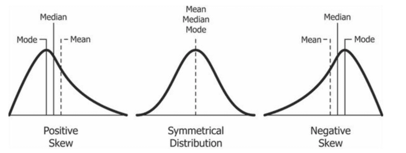
The skewness is the third second. It signifies the asymmetry of the distribution or its lop-sidedness in relation to the distribution’s imply. The skewness impacts the connection between the imply median and mode. A distribution’s skewness could be represented in one among three classes:
- Symmetrical Distribution: The place each side/tails of the distribution are symmetrical. On this class, the worth of the skewness is 0. The imply, median, and mode are the identical in a superbly symmetrical (unimodal) distribution.
- Positively Skewed: The place the appropriate facet/tail of the distribution is longer than the left. That is used to identify and represent outliers with values higher than the imply. This class might also be known as skewed to the appropriate, right-tailed, or right-skewed. Usually, the imply is bigger than the median, which is bigger than the mode (mode < median < imply).
- Negatively Skewed: The place the left facet/tail of the distribution is longer than the appropriate. We use it to establish and signify outliers whose values are lesser than the imply. This class can be known as skewed to the left, left-skewed, or left-tailed. Usually, the mode is bigger than the median, which is bigger than the imply (mode > median > imply).
It’s also possible to use the next easy formulation to search out the skewness:
or
Supply: Creative Commons
Kurtosis E(X^4)
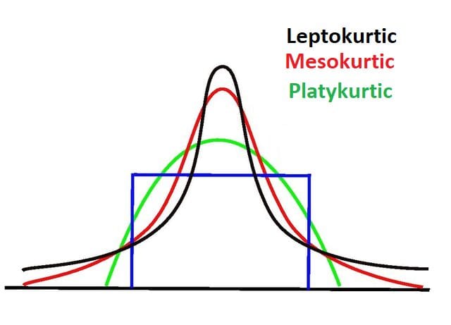
Kurtosis is the fourth second. We use it to measure and point out the prevalence of outliers by utilizing the “tailedness” of the distribution. Thus, kurtosis is most involved with the tails of the distribution. It helps us verify if the distribution is regular or stuffed with excessive values.
Usually, regular distributions have a kurtosis worth of three or an extra kurtosis of 0. Distributions with this sort of kurtosis are known as mesokurtic. A distribution with lighter tails and a kurtosis worth lesser than three (Okay < 3) is known as having destructive kurtosis. In these instances, the distribution is typically broad and flat and known as platykurtic.
Then again, a distribution with heavier tails and a kurtosis worth higher than three (Okay > 3) is known as having a constructive kurtosis. In these instances, the distribution is skinny, has a pointed or excessive peak, and is known as leptokurtic. Excessive kurtosis signifies that the distribution accommodates outliers.
Now that we’ve lined what moments are, we will talk about moment-generating features (MGF).
Second-generating features are in the end features that mean you can generate moments. Within the case the place X is a random variable with a cumulative distribution perform Fx and the place the anticipated variable of t is in shut proximity to some neighborhood of zero, the MGF of X is outlined as:
The place X is discrete, and pi represents the likelihood mass perform (PMF), the definition shall be:
The place X is steady and f(X) represents the probability density function (PDF), the definition will appear to be this:
In instances the place we’re looking for the uncooked second, we should discover the worth of E[xn]. This includes utilizing the nth spinoff of E[etx]. We additionally simplify it by plugging in 0 as the worth of t (t = 0):
Thus, discovering the primary uncooked second (imply) utilizing the MGF with t as 0 appears to be like like this:
You will discover the second uncooked second utilizing the identical method:
You should use Taylor’s Growth (ex=1+x1!+x22!+x33!+…, -∞
MGF affords an alternative choice to integrating the PDF in a steady likelihood distribution to search out its moments. In programming, trying to find the appropriate integration makes algorithms much more advanced and requires extra computing sources, rising the load or run-time of this system. MGFs and their derivations are much more environment friendly at discovering moments.
Discovering the moments of a distribution with out utilizing an MGF is feasible however calculating higher-order moments with out utilizing MGF will get sophisticated. Python’s built-in statistic module comes with a enough record of features that can be utilized to calculate moments from a dataset. Nonetheless, this isn’t the one choice for working with statistical functions in Python.
The above information offers a fundamental exploration of moments and moment-generating features. As a programmer or information scientist, it’s possible you’ll by no means need to manually calculate uncooked moments or attempt to derive central moments manually. In all probability, there are a selection of modules and libraries that try this for you. Nonetheless, it’s all the time vital to grasp what goes on within the background.
Nahla Davies is a software program developer and tech author. Earlier than devoting her work full time to technical writing, she managed — amongst different intriguing issues — to function a lead programmer at an Inc. 5,000 experiential branding group whose purchasers embody Samsung, Time Warner, Netflix, and Sony.
[ad_2]
Source link
