

[ad_1]
Exploring PyMC’s Insights with SHAP Framework by way of an Participating Toy Instance
SHAP values (SHapley Additive exPlanations) are a game-theory-based methodology used to extend the transparency and interpretability of machine studying fashions. Nonetheless, this methodology, together with different machine studying explainability frameworks, has not often been utilized to Bayesian fashions, which offer a posterior distribution capturing uncertainty in parameter estimates as an alternative of level estimates utilized by classical machine studying fashions.
Whereas Bayesian fashions provide a versatile framework for incorporating prior information, adjusting for information limitations, and making predictions, they’re sadly tough to interpret utilizing SHAP. SHAP regards the mannequin as a recreation and every characteristic as a participant in that recreation, however the Bayesian mannequin shouldn’t be a recreation. It’s reasonably an ensemble of video games whose parameters come from the posterior distributions. How can we interpret a mannequin when it’s greater than a recreation?
This text makes an attempt to elucidate a Bayesian mannequin utilizing the SHAP framework by a toy instance. The mannequin is constructed on PyMC, a probabilistic programming library for Python that enables customers to assemble Bayesian fashions with a easy Python API and match them utilizing Markov chain Monte Carlo.
The primary concept is to use SHAP to an ensemble of deterministic fashions generated from a Bayesian community. For every characteristic, we might get hold of one pattern of the SHAP worth from a generated deterministic mannequin. The explainability could be given by the samples of all obtained SHAP values. We’ll illustrate this method with a easy instance.
All of the implementations will be discovered on this notebook .
Dataset
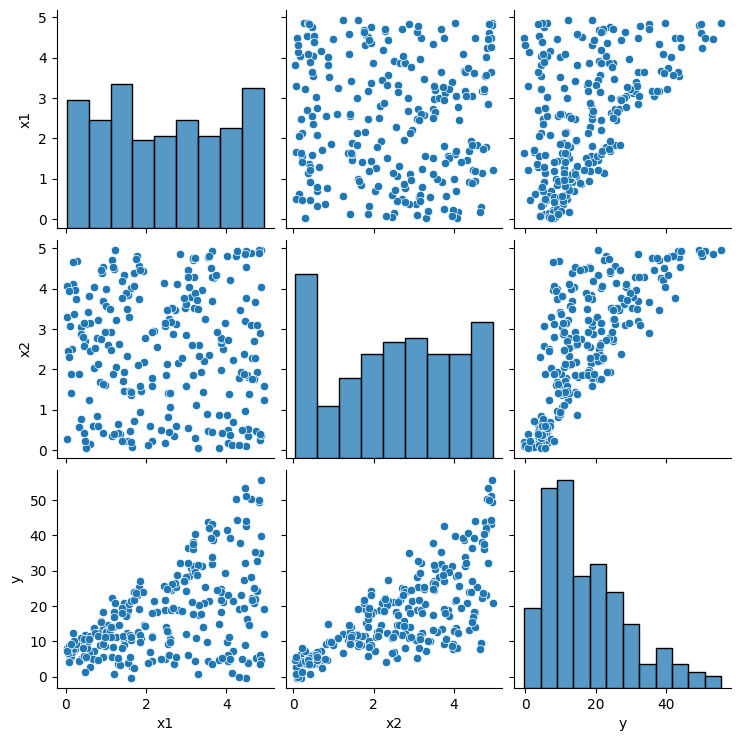
Contemplate the next dataset created by the writer, which accommodates 250 factors: the variable y depends upon x1 and x2, each of which fluctuate between 0 and 5. The picture under illustrates the dataset:

Let’s rapidly discover the info utilizing a pair plot. From this, we will observe the next:
- The variables x1 and x2 are usually not correlated.
- Each variables contribute to the output y to some extent. That’s, a single variable shouldn’t be sufficient to acquire y.

Modelization with PyMC
Let’s construct a Bayesian mannequin with PyMC. With out going into the small print that you will discover in any statistical e book, we’ll merely recall that the coaching technique of Bayesian machine studying fashions includes updating the mannequin’s parameters based mostly on noticed information and prior information utilizing Bayesian rules.
We outline the mannequin’s construction as follows:

Picture by writer: mannequin construction
Defining the priors and chance above, we’ll use the PyMC commonplace sampling algorithm NUTS designed to robotically tune its parameters, such because the step measurement and the variety of leapfrog steps, to attain environment friendly exploration of the goal distribution. It repeats a tree exploration to simulate the trajectory of the purpose within the parameter house and decide whether or not to just accept or reject a pattern. Such iteration stops both when the utmost variety of iterations is reached or the extent of convergence is achieved.
You’ll be able to see within the code under that we arrange the priors, outline the chance, after which run the sampling algorithm utilizing PyMC.
Let’s construct a Bayesian mannequin utilizing PyMC. Bayesian machine studying mannequin coaching includes updating the mannequin’s parameters based mostly on noticed information and prior information utilizing Bayesian rules. We received’t go into element right here, as you will discover it in any statistical e book.
We will outline the mannequin’s construction as proven under:
For the priors and chance outlined above, we’ll use the PyMC commonplace sampling algorithm NUTS. This algorithm is designed to robotically tune its parameters, such because the step measurement and the variety of leapfrog steps, to attain environment friendly exploration of the goal distribution. It repeats a tree exploration to simulate the trajectory of the purpose within the parameter house and decide whether or not to just accept or reject a pattern. The iteration stops both when the utmost variety of iterations is reached or the extent of convergence is achieved.
Within the code under, we arrange the priors, outline the chance, after which run the sampling algorithm utilizing PyMC.
with pm.Mannequin() as mannequin:# Set priors.
intercept=pm.Uniform(identify="intercept",decrease=-10, higher=10)
x1_slope=pm.Uniform(identify="x1_slope",decrease=-5, higher=5)
x2_slope=pm.Uniform(identify="x2_slope",decrease=-5, higher=5)
interaction_slope=pm.Uniform(identify="interaction_slope",decrease=-5, higher=5)
sigma=pm.Uniform(identify="sigma", decrease=1, higher=5)
# Set likelhood.
chance = pm.Regular(identify="y", mu=intercept + x1_slope*x1+x2_slope*x2+interaction_slope*x1*x2,
sigma=sigma, noticed=y)
# Configure sampler.
hint = pm.pattern(5000, chains=5, tune=1000, target_accept=0.87, random_seed=SEED)
The hint plot under shows the posteriors of the parameters within the mannequin.

We now wish to implement SHAP on the mannequin described above. Notice that for a given enter (x1, x2), the mannequin’s output y is a likelihood conditional on the parameters. Thus, we will get hold of a deterministic mannequin and corresponding SHAP values for all options by drawing one pattern from the obtained posteriors. Alternatively, if we draw an ensemble of parameter samples, we are going to get an ensemble of deterministic fashions and, due to this fact, samples of SHAP values for all options.
The posteriors will be obtained utilizing the next code, the place we draw 200 samples per chain:
with mannequin:
idata = pm.sample_prior_predictive(samples=200, random_seed=SEED)
idata.prolong(pm.pattern(200, tune=2000, random_seed=SEED)right here
Right here is the desk of the info variables from the posteriors:

Subsequent, we compute one pair of SHAP values for every drawn pattern of mannequin parameters. The code under loops over the parameters, defines one mannequin for every parameter pattern, and computes the SHAP values of x_test=(2,3) of curiosity.
background=np.hstack((x1.reshape((250,1)),x2.reshape((250,1))))
shap_values_list=[]
x_test=np.array([2,3]).reshape((-1,2))
for i in vary(len(pos_intercept)):
mannequin=SimpleModel(intercept=pos_intercept[i],
x1_slope=pos_x1_slope[i],
x2_slope=pos_x2_slope[i],
interaction_slope=pos_interaction_slope[i],
sigma=pos_sigma[i])
explainer = shap.Explainer(mannequin.predict, background)
shap_values = explainer(x_test)
shap_values_list.append(shap_values.values)
The ensuing ensemble of the two-dimensional SHAP values of the enter is proven under:

From the plot above, we will infer the next:
- The SHAP values of each dimensions kind kind of a standard distribution.
- The primary dimension has a constructive contribution (-1.75 as median) to the mannequin, whereas the second has a destructive contribution (3.45 as median). Nonetheless, the second dimension’s contribution has a much bigger absolute worth.
This text explores using SHAP values, a game-theory-based methodology for rising transparency and interpretability of machine studying fashions, in Bayesian fashions. A toy instance is used to display how SHAP will be utilized to a Bayesian community.
Please word that SHAP is model-agnostic. Subsequently, with adjustments to its implementation, it could be potential to use SHAP on to the Bayesian mannequin itself sooner or later.
[ad_2]
Source link
