


[ad_1]

Picture by Writer
As information scientists, we depend on statistical evaluation to crawl info from the info in regards to the relationships between totally different variables to reply questions, which is able to assist companies and people to make the best choices. Nonetheless, some statistical phenomena might be counterintuitive, presumably resulting in paradoxes and biases in our evaluation, which is able to damage our evaluation.
These paradoxes I’ll clarify to you’re straightforward to know and don’t embody complicated formulation.
On this article, we are going to discover 5 statistical paradoxes information scientists ought to pay attention to: the accuracy paradox, the False Optimistic Paradox, Gambler’s Fallacy, Simpson’s Paradox, and Berkson’s paradox.
Every of those paradoxes often is the potential motive for getting the unreliable results of your evaluation.
Picture by Writer
We’ll focus on the definitions of those paradoxes and real-life examples as an example how these paradoxes can occur in real-world information evaluation. Understanding these paradoxes will make it easier to take away doable roadblocks to dependable statistical evaluation.
So, with out additional ado, let’s dive into the world of paradoxes with Accuracy Paradox.

Picture by Writer
Accuracy exhibits that accuracy is just not a very good analysis metric on the subject of classifying.
Suppose you’re analyzing a dataset that incorporates 1000 affected person metrics. You wish to catch a uncommon form of illness, which is able to finally be proven itself in 5% of the inhabitants. So total, you need to discover 50 folks in 1000.
Even if you happen to at all times say that the folks do not need a illness, your accuracy might be 95%. And your mannequin cannot catch a single sick particular person on this cluster. (0/50)
Digits Information Set
Let’s clarify this by giving an instance from well-known digits information set.
This information set incorporates hand-written numbers from 0 to 9.

Picture by Writer
It’s a easy multilabel classification job, however it can be interpreted as picture recognition for the reason that numbers are offered as photographs.
Now we are going to load these information units and reshape the info set to use the machine studying mannequin. I’m skipping explaining these components as a result of you may additionally be conversant in this half. If not, strive looking digit information set or MNIST information set. MNIST information set additionally incorporates the identical form of information, however the form is greater than this one.
Alright, let’s proceed.
Now we attempt to predict if the quantity is 6 or not. To do this, we are going to outline a classifier that predicts not 6. Let’s have a look at the cross-validation rating of this classifier.
from sklearn import datasets
from sklearn.model_selection import train_test_split
from sklearn.model_selection import cross_val_score
from sklearn.base import BaseEstimator
import numpy as np

digits = datasets.load_digits()
n_samples = len(digits.photographs)
information = digits.photographs.reshape((n_samples, -1))
x_train, x_test, y_train, y_test = train_test_split(
    information, digits.goal, test_size=0.5, shuffle=False
)
y_train_6 = y_train == 6

from sklearn.base import BaseEstimator


class DumbClassifier(BaseEstimator):
    def match(self, X, y=None):
        move

    def predict(self, X):
        return np.zeros((len(X), 1), dtype=bool)


dumb_clf = DumbClassifier()

cross_val_score(dumb_clf, x_train, y_train_6, cv=3, scoring="accuracy")
Right here the outcomes might be as the next.

What does it imply? Which means even if you happen to create an estimator that can by no means estimate 6 and you place that in your mannequin, the accuracy might be over 90%. Why? As a result of 9 different numbers exist in our dataset. So if you happen to say the quantity is just not 6, you’ll be proper 9/10 occasions.
This exhibits it’s necessary to decide on your analysis metrics rigorously. Accuracy is just not a good selection if you wish to consider your classification duties. You must select precision or recall.
What are these? They arrive up within the False Optimistic Paradox, so proceed studying.

Picture by Writer
Now, the false constructive paradox is a statistical phenomenon that may happen after we check for the presence of a uncommon occasion or situation.
Additionally it is often known as the “base charge fallacy” or “base charge neglect”.
This paradox means there are extra false constructive outcomes than constructive outcomes when testing uncommon occasions.
Let’s have a look at the instance from Information Science.
Fraud Detection

Picture by Writer
Think about you’re engaged on an ML mannequin to detect fraudulent bank card transactions. The dataset you’re working with consists of a lot of regular (non-fraudulent) transactions and a small variety of fraudulent transactions. But whenever you deploy your mannequin in the true world, you discover that it produces a lot of false positives.
After additional investigation, you understand that the prevalence of fraudulent transactions in the true world is far decrease than within the coaching dataset.
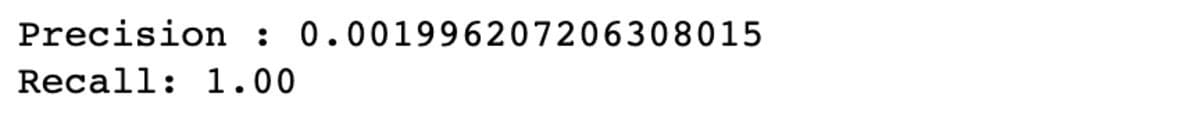
Let’s say 1/10,000 transactions might be fraudulent, and suppose the check additionally has a 5% charge of false positives.
TP = 1 out of 10,000
FP = 10,000*(100-40)/100*0,05 = 499,95 out of 9,999
So when a fraudulent transaction is discovered, what’s the chance that it truly is a fraudulent transaction?
P = 1/500,95 =0,001996
The result’s almost 0.2%. It means when the occasion will get flagged as fraudulent, there may be solely a 0.2% chance that it truly is a fraudulent occasion.
And that could be a false constructive paradox.
Right here is the way to implement it in Python code.
import pandas as pd
import numpy as np

# Variety of regular transactions
normal_count = 9999

# Variety of fraudulent transactions
true_positive = 1

# Variety of regular transactions flagged as fraudulent by the mannequin
false_positives = 499.95

# Variety of fraudulent transactions flagged as regular by the mannequin
false_negatives = 0

# Calculate precision
precision = (true_positive) / true_positive + false_positives
print(f"Precision: {precision:.2f}")

# Calculate recall
recall = (fraud_count) / fraud_count + false_negatives
print(f"Recall: {recall:.2f}")

# Calculate accuracy
accuracy = (
    normal_count - false_positives + fraud_count - false_negatives
) / (normal_count + fraud_count)
print(f"Accuracy: {accuracy:.2f}")
You’ll be able to see that the recall is actually excessive, but the precision could be very low.
To grasp why techniques try this, let me clarify the precision/recall and precision/recall tradeoff.
Recall (true constructive charge) can be known as sensitivity. You must first discover the positives and discover the speed of true positives amongst them.
Recall = TP / TP + FP
Precision is the accuracy of constructive prediction.
Precision = TP / TP + FN
Let’s say you need a classifier that can do sentiment evaluation and predict whether or not the feedback might be constructive or destructive. You may want a classifier that has excessive recall (it accurately identifies a excessive proportion of constructive or destructive feedback). Nonetheless, to have a better recall, you ought to be okay with having a decrease precision (misclassification of constructive feedback) as a result of it’s extra necessary to delete destructive feedback than delete a couple of constructive feedback often.
Alternatively, if you wish to construct a spam classifier, you may want a classifier that has excessive precision. It accurately identifies excessive percentages of spam, but every so often, it permits spam as a result of it’s extra necessary to maintain necessary mail.
Now in our case, to discover a fraudulent transaction, you sacrifice getting many errors that aren’t fraudulent, but if you happen to accomplish that, you need to take precautions, too, like in banking techniques. After they detect fraudulent transactions, they start to do additional investigations to be completely positive.
Sometimes they ship a message to your cellphone or electronic mail for additional approval when doing a transaction over a preset restrict, and so forth.
In the event you enable your mannequin to have a False destructive, then your recall might be legislation. But, if you happen to enable your mannequin to have a False constructive, your Precision might be low.
As an information scientist, you need to alter your mannequin or add a step to make additional investigations as a result of there could be a variety of False Positives.

Picture by Writer
Gambler’s fallacy, also referred to as the Monte Carlo fallacy, is the mistaken perception that if an occasion occurs extra incessantly than its regular chance, it can occur extra usually within the following trials.
Let’s have a look at the instance from the Information Science discipline.
Buyer Churn

Picture by Writer
Think about that you’re constructing a machine studying mannequin to foretell whether or not the shopper will churn based mostly on their previous habits.
Now, you collected many various kinds of information, together with the variety of prospects interacting with the companies, the size of time they’ve been a buyer, the variety of complaints they’ve made, and extra.
At this level, you might be tempted to assume a buyer who has been with the service for a very long time is much less prone to churn as a result of they’ve proven a dedication to the service previously.
Nonetheless, that is an instance of a gambler’s fallacy as a result of the chance of a buyer churning is just not influenced by the size of time they’ve been a buyer.
The chance of churn is set by a variety of things, together with the standard of the service, the shopper’s satisfaction with the service, and extra of those elements.
So if you happen to construct a machine studying mannequin, watch out explicitly to not create a column that features the size of a buyer and attempt to clarify the mannequin through the use of that. At this level, you need to understand that this would possibly damage your mannequin resulting from Gambler’s fallacy.
Now, this was a conceptual instance. Let’s attempt to clarify this by giving an instance of the coin toss.
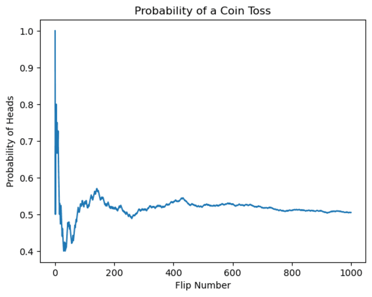
Let’s first have a look at the adjustments within the coin toss chance. You could be tempted to assume that if the coin has come up heads a number of occasions, the likelihood sooner or later will diminish. That is truly an incredible instance of the gambler’s fallacy.
As you may see, at first, the likelihood fluctuated. But when the variety of flips will increase, the potential for getting heads will converge to 0.5.
import random
import matplotlib.pyplot as plt

# Arrange the plot
plt.xlabel("Flip Quantity")
plt.ylabel("Likelihood of Heads")

# Initialize variables
num_flips = 1000
num_heads = 0
chances = []

# Simulate the coin flips
for i in vary(num_flips):
    if (
        random.random() > 0.5
    ):  # random() generates a random float between 0 and 1
        num_heads += 1
    chance = num_heads / (i + 1)  # Calculate the chance of heads
    chances.append(chance)  # Report the chance
# Plot the outcomes
plt.plot(chances)
plt.present()
Now, let’s see the output.
Picture by Writer
It’s apparent that chance fluctuates over time, however because of this, it can converge towards 0.5.
This instance exhibits Gambler’s fallacy as a result of the outcomes of earlier flips don’t affect the chance of getting heads on any given flip. The chance stays fastened at 50% no matter what has occurred previously.

Picture by Roland Steinmann from Pixabay
This paradox occurs when the connection between two variables seems to vary when information is aggregated.
Now, to clarify this paradox, let’s use the built-in information set in seaborn, ideas.
Ideas

Picture by Writer
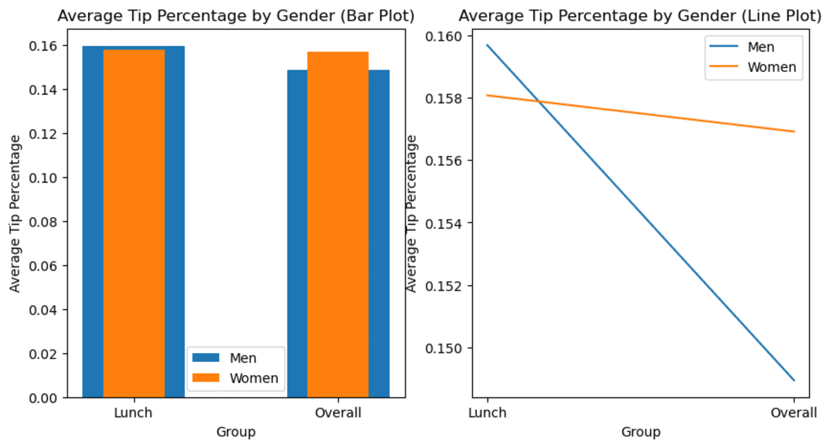
To clarify Simpson’s paradox, we are going to calculate the imply of the common ideas men and women made throughout lunch and total through the use of the information information set. The guidelines dataset incorporates information on ideas given by prospects at a restaurant, like complete ideas, intercourse, day, time, and extra.
The guidelines dataset is a group of knowledge on ideas given by prospects at a restaurant. It consists of info such because the tip quantity, the gender of the shopper, the day of the week, and the time of day. The dataset can be utilized to investigate prospects’ tipping habits and establish developments within the information.
import seaborn as sns

# Load the information dataset
ideas = sns.load_dataset("ideas")

# Calculate the tip proportion for women and men at lunch
men_lunch_tip_pct = (
    ideas[(tips["sex"] == "Male") & (ideas["time"] == "Lunch")]["tip"].imply()
    / ideas[(tips["sex"] == "Male") & (ideas["time"] == "Lunch")][
        "total_bill"
    ].imply()
)
women_lunch_tip_pct = (
    ideas[(tips["sex"] == "Feminine") & (ideas["time"] == "Lunch")]["tip"].imply()
    / ideas[(tips["sex"] == "Feminine") & (ideas["time"] == "Lunch")][
        "total_bill"
    ].imply()
)

# Calculate the general tip proportion for women and men
men_tip_pct = (
    ideas[tips["sex"] == "Male"]["tip"].imply()
    / ideas[tips["sex"] == "Male"]["total_bill"].imply()
)
women_tip_pct = (
    ideas[tips["sex"] == "Feminine"]["tip"].imply()
    / ideas[tips["sex"] == "Feminine"]["total_bill"].imply()
)

# Create an information body with the common tip percentages
information = {
    "Lunch": [men_lunch_tip_pct, women_lunch_tip_pct],
    "Total": [men_tip_pct, women_tip_pct],
}
index = ["Men", "Women"]
df = pd.DataFrame(information, index=index)
df
Alright, right here is our information body.
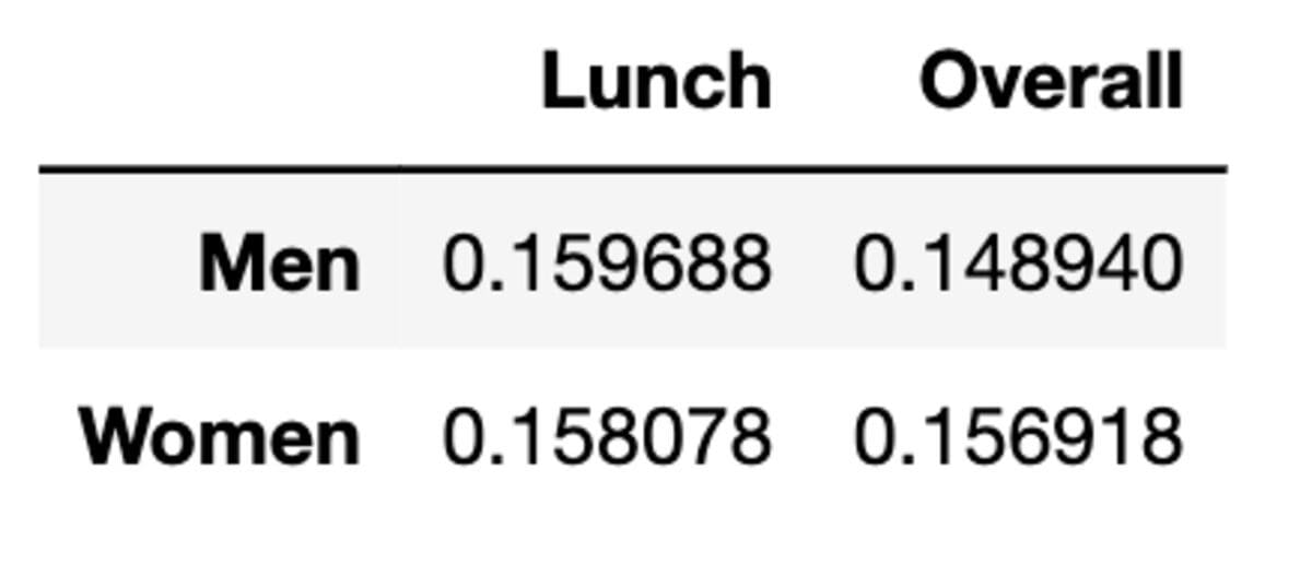
As we are able to see, the common tip is greater on the subject of lunch between women and men. But when information is aggregated, the imply is modified.
Let’s see the bar chart to see the adjustments.
import matplotlib.pyplot as plt

# Set the group labels
labels = ["Lunch", "Overall"]

# Set the bar heights
men_heights = [men_lunch_tip_pct, men_tip_pct]
women_heights = [women_lunch_tip_pct, women_tip_pct]

# Create a determine with two subplots
fig, (ax1, ax2) = plt.subplots(1, 2, figsize=(10, 5))

# Create the bar plot
ax1.bar(labels, men_heights, width=0.5, label="Males")
ax1.bar(labels, women_heights, width=0.3, label="Girls")
ax1.set_title("Common Tip Proportion by Gender (Bar Plot)")
ax1.set_xlabel("Group")
ax1.set_ylabel("Common Tip Proportion")
ax1.legend()

# Create the road plot
ax2.plot(labels, men_heights, label="Males")
ax2.plot(labels, women_heights, label="Girls")
ax2.set_title("Common Tip Proportion by Gender (Line Plot)")
ax2.set_xlabel("Group")
ax2.set_ylabel("Common Tip Proportion")
ax2.legend()

# Present the plot
plt.present()
Right here is the output.
Picture by Writer
Now, as you may see, the common adjustments as information are aggregated. Instantly, you’ve information exhibiting that total, girls tip greater than males.
What’s the catch?
When observing the pattern from the subset model and extracting which means from them, watch out to not neglect to test whether or not this pattern continues to be the case for the entire information set or not. As a result of as you may see, there may not be the case in particular circumstances. This may lead a Information Scientist to make a misjudgment, resulting in a poor (enterprise) determination.
Berkson’s Paradox is a statistical paradox that occurs when two variables correlated to one another in information, but when the info will subsetted, or grouped, this correlation is just not noticed & modified.
In easy phrases, Berkson’s Paradox is when a correlation seems to be totally different in several subgroups of the info.
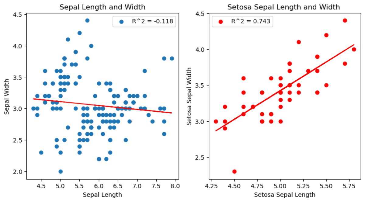
Now let’s look into it by analyzing the Iris dataset.
Iris Information set

Picture by Writer
The Iris dataset is a generally used dataset in machine studying and statistics. It incorporates information for various observations of irises, together with their petal and sepal size and width and the flower species noticed.
Right here, we are going to draw two graphs exhibiting the connection between sepal size and width. However within the second graph, we filter the species as a setosa.
import seaborn as sns
import matplotlib.pyplot as plt
from scipy.stats import linregress

# Load the iris information set
df = sns.load_dataset("iris")

# Subset the info to solely embody setosa species
df_s = df[df["species"] == "setosa"]

# Create a determine with two subplots
fig, (ax1, ax2) = plt.subplots(1, 2, figsize=(10, 5))

# Plot the connection between sepal size and width.
slope, intercept, r_value, p_value, std_err = linregress(
    df["sepal_length"], df["sepal_width"]
)
ax1.scatter(df["sepal_length"], df["sepal_width"])
ax1.plot(
    df["sepal_length"],
    intercept + slope * df["sepal_length"],
    "r",
    label="fitted line",
)
ax1.set_xlabel("Sepal Size")
ax1.set_ylabel("Sepal Width")
ax1.set_title("Sepal Size and Width")
ax1.legend([f"R^2 = {r_value:.3f}"])

# Plot the connection between setosa sepal size and width for setosa.
slope, intercept, r_value, p_value, std_err = linregress(
    df_s["sepal_length"], df_s["sepal_width"]
)
ax2.scatter(df_s["sepal_length"], df_s["sepal_width"])
ax2.plot(
    df_s["sepal_length"],
    intercept + slope * df_s["sepal_length"],
    "r",
    label="fitted line",
)
ax2.set_xlabel("Setosa Sepal Size")
ax2.set_ylabel("Setosa Sepal Width")
ax2.set_title("Setosa Sepal Size and Width ")
ax2.legend([f"R^2 = {r_value:.3f}"])

# Present the plot
plt.present()
You’ll be able to see the adjustments between sepal size and throughout the setosa species. Really, it exhibits a special correlation than different species.
Picture by Writer
Additionally, you may see that setosa’s totally different correlation within the first graph.
Within the second graph, you may see that the correlation between sepal width and sepal size has modified. When analyzing all information set, it exhibits that when sepal size will increase, sepal width decreases. Nonetheless, if we begin analyzing by deciding on setosa species, the correlation is now constructive and exhibits that when sepal width will increase, sepal size will increase as effectively.
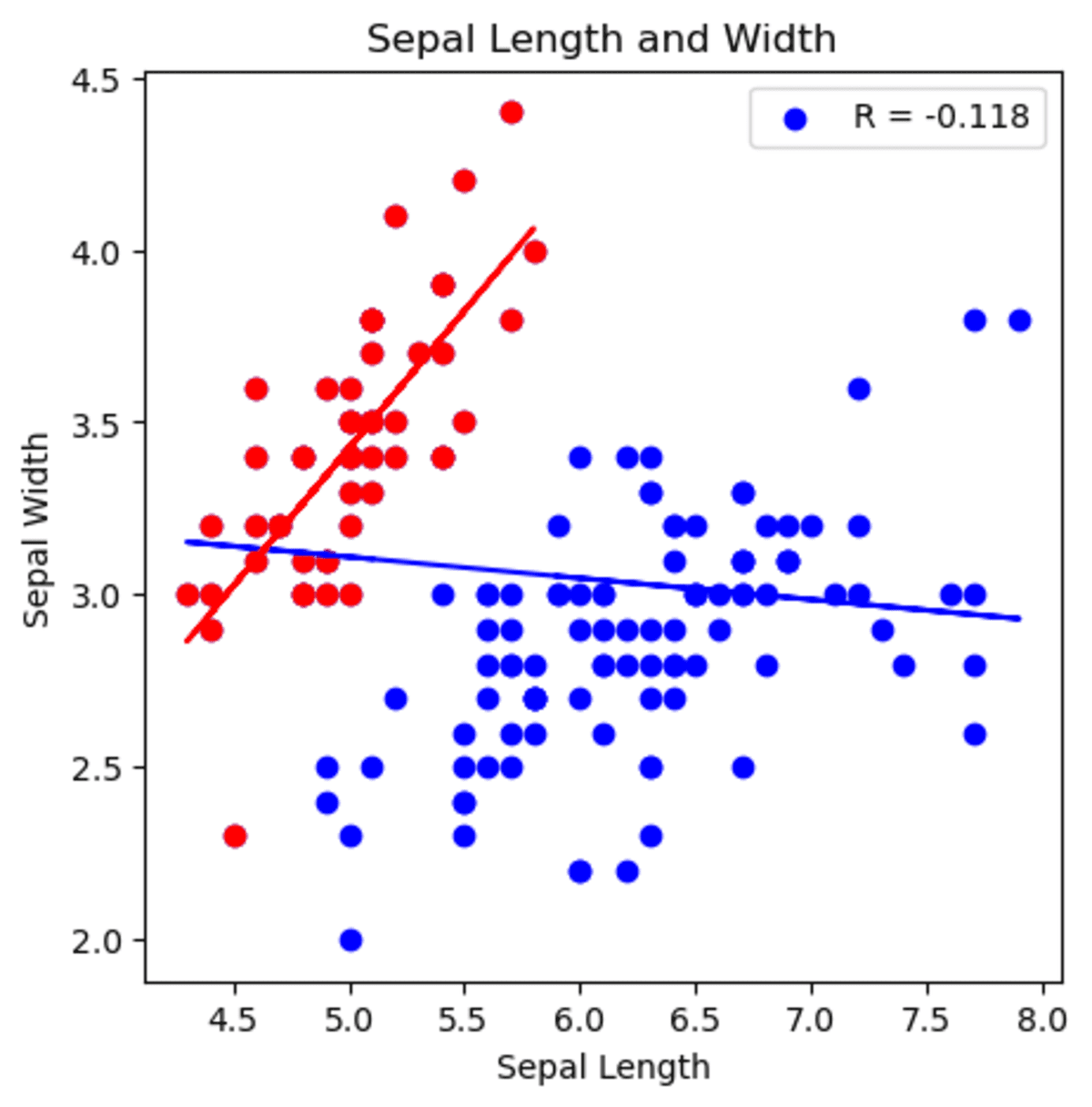
import seaborn as sns
import matplotlib.pyplot as plt
from scipy.stats import linregress

# Load the information information set
df = sns.load_dataset("iris")

# Subset the info to solely embody setosa species
df_s = df[df["species"] == "setosa"]

# Create a determine with two subplots
fig, ax1 = plt.subplots(figsize=(5, 5))

# Plot the connection between sepal size and width.
slope, intercept, r_value_1, p_value, std_err = linregress(
    df["sepal_length"], df["sepal_width"]
)
ax1.scatter(df["sepal_length"], df["sepal_width"], coloration="blue")
ax1.plot(
    df["sepal_length"],
    intercept + slope * df["sepal_length"],
    "b",
    label="fitted line",
)

# Plot the connection between setosa sepal size and width for setosa.
slope, intercept, r_value_2, p_value, std_err = linregress(
    df_s["sepal_length"], df_s["sepal_width"]
)
ax1.scatter(df_s["sepal_length"], df_s["sepal_width"], coloration="purple")
ax1.plot(
    df_s["sepal_length"],
    intercept + slope * df_s["sepal_length"],
    "r",
    label="fitted line",
)

ax1.set_xlabel("Sepal Size")
ax1.set_ylabel("Sepal Width")
ax1.set_title("Sepal Size and Width")
ax1.legend([f"R = {r_value_1:.3f}"])
Right here is the graph.
Picture by Writer
You’ll be able to see that beginning by analyzing with setosa and generalizing the sepal width and size correlation will lead you to make a false assertion based on your evaluation.
On this article, we examined 5 statistical paradoxes that information scientists ought to pay attention to with a purpose to do correct evaluation. Let’s suppose you assume that you simply discovered a pattern in your information set, which signifies that when sepal size will increase, sepal width will increase as effectively. But when wanting on the complete information set, it’s truly the full reverse.
Otherwise you could be assessing your classification fashions by wanting on the accuracy. You see that even the mannequin that does nothing can obtain over 90% accuracy. In the event you tried to judge your mannequin with accuracy and do evaluation accordingly, take into consideration what number of miscalculations you can also make.
By understanding these paradoxes, we are able to take steps to keep away from widespread pitfalls and enhance the reliability of our statistical evaluation. It’s additionally good to method information evaluation with a wholesome dose of skepticism and keep away from potential paradoxes and limitations in your analyses.
In conclusion, these paradoxes are necessary for Information Scientists on the subject of high-level evaluation, as being conscious of them can enhance the accuracy and reliability of our evaluation. We additionally suggest this “Statistics Cheat Sheet” that may make it easier to perceive the necessary phrases and equations for statistics and chance and can assist you in your subsequent information science interview.
Thanks for studying!
Nate Rosidi is an information scientist and in product technique. He is additionally an adjunct professor instructing analytics, and is the founding father of StrataScratch, a platform serving to information scientists put together for his or her interviews with actual interview questions from prime firms. Join with him on Twitter: StrataScratch or LinkedIn.
[ad_2]
Source link
