A Gentle Introduction to Graph Neural Networks

This text is one in every of two Distill publications about graph neural networks. Check out Understanding Convolutions on Graphs to grasp how convolutions over photographs generalize naturally to convolutions over graphs.

Graphs are throughout us; actual world objects are sometimes outlined when it comes to their connections to different issues. A set of objects, and the connections between them, are naturally expressed as a graph. Researchers have developed neural networks that function on graph knowledge (referred to as graph neural networks, or GNNs) for over a decade. Current developments have elevated their capabilities and expressive energy. We’re beginning to see sensible functions in areas equivalent to antibacterial discovery , physics simulations , faux information detection , site visitors prediction and suggestion techniques .

This text explores and explains trendy graph neural networks. We divide this work into 4 components. First, we take a look at what sort of knowledge is most naturally phrased as a graph, and a few widespread examples. Second, we discover what makes graphs totally different from different varieties of knowledge, and a number of the specialised selections we’ve to make when utilizing graphs. Third, we construct a contemporary GNN, strolling by every of the components of the mannequin, beginning with historic modeling improvements within the subject. We transfer regularly from a bare-bones implementation to a state-of-the-art GNN mannequin. Fourth and eventually, we offer a GNN playground the place you’ll be able to mess around with a real-word process and dataset to construct a stronger instinct of how every part of a GNN mannequin contributes to the predictions it makes.

To begin, let’s set up what a graph is. A graph represents the relations (edges) between a group of entities (nodes).

To additional describe every node, edge or the complete graph, we will retailer info in every of those items of the graph.

We will moreover specialize graphs by associating directionality to edges (directed, undirected).

Graphs are very versatile knowledge constructions, and if this appears summary now, we’ll make it concrete with examples within the subsequent part.

Graphs and the place to search out them

You’re in all probability already acquainted with some varieties of graph knowledge, equivalent to social networks. Nevertheless, graphs are an especially highly effective and normal illustration of knowledge, we’ll present two varieties of knowledge that you simply won’t assume may very well be modeled as graphs: photographs and textual content. Though counterintuitive, one can study extra concerning the symmetries and construction of photographs and textual content by viewing them as graphs,, and construct an instinct that may assist perceive different much less grid-like graph knowledge, which we’ll focus on later.

Pictures as graphs

We sometimes consider photographs as rectangular grids with picture channels, representing them as arrays (e.g., 244x244x3 floats). One other method to think about photographs is as graphs with common construction, the place every pixel represents a node and is related by way of an edge to adjoining pixels. Every non-border pixel has precisely 8 neighbors, and the knowledge saved at every node is a three-dimensional vector representing the RGB worth of the pixel.

A method of visualizing the connectivity of a graph is thru its adjacency matrix. We order the nodes, on this case every of 25 pixels in a easy 5×5 picture of a smiley face, and fill a matrix of $n_{nodes} occasions n_{nodes}$ with an entry if two nodes share an edge. Notice that every of those three representations under are totally different views of the identical piece of knowledge.

Textual content as graphs

We will digitize textual content by associating indices to every character, phrase, or token, and representing textual content as a sequence of those indices. This creates a easy directed graph, the place every character or index is a node and is related by way of an edge to the node that follows it.

In fact, in apply, this isn’t often how textual content and pictures are encoded: these graph representations are redundant since all photographs and all textual content can have very common constructions. As an example, photographs have a banded construction of their adjacency matrix as a result of all nodes (pixels) are related in a grid. The adjacency matrix for textual content is only a diagonal line, as a result of every phrase solely connects to the prior phrase, and to the subsequent one.

Graph-valued knowledge within the wild

Graphs are a useful gizmo to explain knowledge you would possibly already be acquainted with. Let’s transfer on to knowledge which is extra heterogeneously structured. In these examples, the variety of neighbors to every node is variable (versus the fastened neighborhood dimension of photographs and textual content). This knowledge is tough to phrase in every other method in addition to a graph.

Molecules as graphs. Molecules are the constructing blocks of matter, and are constructed of atoms and electrons in 3D house. All particles are interacting, however when a pair of atoms are caught in a steady distance from one another, we are saying they share a covalent bond. Totally different pairs of atoms and bonds have totally different distances (e.g. single-bonds, double-bonds). It’s a really handy and customary abstraction to explain this 3D object as a graph, the place nodes are atoms and edges are covalent bonds. Listed below are two widespread molecules, and their related graphs.

Social networks as graphs. Social networks are instruments to review patterns in collective behaviour of individuals, establishments and organizations. We will construct a graph representing teams of individuals by modelling people as nodes, and their relationships as edges.

In contrast to picture and textual content knowledge, social networks shouldn’t have an identical adjacency matrices.

Quotation networks as graphs. Scientists routinely cite different scientists’ work when publishing papers. We will visualize these networks of citations as a graph, the place every paper is a node, and every directed edge is a quotation between one paper and one other. Moreover, we will add details about every paper into every node, equivalent to a phrase embedding of the summary. (see ,  , ).

Different examples. In pc imaginative and prescient, we generally need to tag objects in visible scenes. We will then construct graphs by treating these objects as nodes, and their relationships as edges. Machine learning models, programming code and math equations will also be phrased as graphs, the place the variables are nodes, and edges are operations which have these variables as enter and output. You would possibly see the time period “dataflow graph” utilized in a few of these contexts.

The construction of real-world graphs can range significantly between various kinds of knowledge — some graphs have many nodes with few connections between them, or vice versa. Graph datasets can range broadly (each inside a given dataset, and between datasets) when it comes to the variety of nodes, edges, and the connectivity of nodes.

What varieties of issues have graph structured knowledge?

Now we have described some examples of graphs within the wild, however what duties can we need to carry out on this knowledge? There are three normal varieties of prediction duties on graphs: graph-level, node-level, and edge-level.

In a graph-level process, we predict a single property for an entire graph. For a node-level process, we predict some property for every node in a graph. For an edge-level process, we need to predict the property or presence of edges in a graph.

For the three ranges of prediction issues described above (graph-level, node-level, and edge-level), we’ll present that the entire following issues might be solved with a single mannequin class, the GNN. However first, let’s take a tour by the three courses of graph prediction issues in additional element, and supply concrete examples of every.

Graph-level process

In a graph-level process, our objective is to foretell the property of a complete graph. For instance, for a molecule represented as a graph, we’d need to predict what the molecule smells like, or whether or not it can bind to a receptor implicated in a illness.

That is analogous to picture classification issues with MNIST and CIFAR, the place we need to affiliate a label to a complete picture. With textual content, the same downside is sentiment evaluation the place we need to determine the temper or emotion of a complete sentence without delay.

Node-level process

Node-level duties are involved with predicting the identification or position of every node inside a graph.

A basic instance of a node-level prediction downside is Zach’s karate membership. The dataset is a single social community graph made up of people which have sworn allegiance to one in every of two karate golf equipment after a political rift. Because the story goes, a feud between Mr. Hello (Teacher) and John H (Administrator) creates a schism within the karate membership. The nodes symbolize particular person karate practitioners, and the perimeters symbolize interactions between these members outdoors of karate. The prediction downside is to categorise whether or not a given member turns into loyal to both Mr. Hello or John H, after the feud. On this case, distance between a node to both the Teacher or Administrator is extremely correlated to this label.

Following the picture analogy, node-level prediction issues are analogous to picture segmentation, the place we try to label the position of every pixel in a picture. With textual content, the same process can be predicting the parts-of-speech of every phrase in a sentence (e.g. noun, verb, adverb, and so forth).

Edge-level process

The remaining prediction downside in graphs is edge prediction.

One instance of edge-level inference is in picture scene understanding. Past figuring out objects in a picture, deep studying fashions can be utilized to foretell the connection between them. We will phrase this as an edge-level classification: given nodes that symbolize the objects within the picture, we want to predict which of those nodes share an edge or what the worth of that edge is. If we want to uncover connections between entities, we may take into account the graph totally related and primarily based on their predicted worth prune edges to reach at a sparse graph.

The challenges of utilizing graphs in machine studying

So, how can we go about fixing these totally different graph duties with neural networks? Step one is to consider how we’ll symbolize graphs to be suitable with neural networks.

Machine studying fashions sometimes take rectangular or grid-like arrays as enter. So, it’s not instantly intuitive symbolize them in a format that’s suitable with deep studying. Graphs have as much as 4 varieties of info that we’ll doubtlessly need to use to make predictions: nodes, edges, global-context and connectivity. The primary three are comparatively easy: for instance, with nodes we will type a node characteristic matrix $N$ by assigning every node an index $i$ and storing the characteristic for $node_i$ in $N$. Whereas these matrices have a variable variety of examples, they are often processed with none particular strategies.

Nevertheless, representing a graph’s connectivity is extra sophisticated. Maybe the obvious alternative can be to make use of an adjacency matrix, since that is simply tensorisable. Nevertheless, this illustration has just a few drawbacks. From the example dataset table, we see the variety of nodes in a graph might be on the order of hundreds of thousands, and the variety of edges per node might be extremely variable. Typically, this results in very sparse adjacency matrices, that are space-inefficient.

One other downside is that there are lots of adjacency matrices that may encode the identical connectivity, and there’s no assure that these totally different matrices would produce the identical end in a deep neural community (that’s to say, they don’t seem to be permutation invariant).

For instance, the Othello graph from earlier than might be described equivalently with these two adjacency matrices. It will also be described with each different potential permutation of the nodes.

The instance under exhibits each adjacency matrix that may describe this small graph of 4 nodes. That is already a major variety of adjacency matrices–for bigger examples like Othello, the quantity is untenable.

One elegant and memory-efficient method of representing sparse matrices is as adjacency lists. These describe the connectivity of edge $e_k$ between nodes $n_i$ and $n_j$ as a tuple (i,j) within the k-th entry of an adjacency record. Since we count on the variety of edges to be a lot decrease than the variety of entries for an adjacency matrix ($n_{nodes}^2$), we keep away from computation and storage on the disconnected components of the graph.

To make this notion concrete, we will see how info in several graphs is likely to be represented beneath this specification:

It needs to be famous that the determine makes use of scalar values per node/edge/international, however most sensible tensor representations have vectors per graph attribute. As a substitute of a node tensor of dimension $[n_{nodes}]$ we can be coping with node tensors of dimension $[n_{nodes}, node_{dim}]$. Identical for the opposite graph attributes.

Graph Neural Networks

Now that the graph’s description is in a matrix format that’s permutation invariant, we’ll describe utilizing graph neural networks (GNNs) to resolve graph prediction duties. A GNN is an optimizable transformation on all attributes of the graph (nodes, edges, global-context) that preserves graph symmetries (permutation invariances). We’re going to construct GNNs utilizing the “message passing neural community” framework proposed by Gilmer et al. utilizing the Graph Nets structure schematics launched by Battaglia et al. GNNs undertake a “graph-in, graph-out” structure which means that these mannequin sorts settle for a graph as enter, with info loaded into its nodes, edges and global-context, and progressively remodel these embeddings, with out altering the connectivity of the enter graph.

The best GNN

With the numerical illustration of graphs that we’ve constructed above (with vectors as an alternative of scalars), we at the moment are able to construct a GNN. We are going to begin with the best GNN structure, one the place we study new embeddings for all graph attributes (nodes, edges, international), however the place we don’t but use the connectivity of the graph.

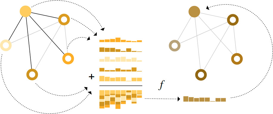
This GNN makes use of a separate multilayer perceptron (MLP) (or your favourite differentiable mannequin) on every part of a graph; we name this a GNN layer. For every node vector, we apply the MLP and get again a realized node-vector. We do the identical for every edge, studying a per-edge embedding, and likewise for the global-context vector, studying a single embedding for the complete graph.

As is widespread with neural networks modules or layers, we will stack these GNN layers collectively.

As a result of a GNN doesn’t replace the connectivity of the enter graph, we will describe the output graph of a GNN with the identical adjacency record and the identical variety of characteristic vectors because the enter graph. However, the output graph has up to date embeddings, because the GNN has up to date every of the node, edge and global-context representations.

GNN Predictions by Pooling Info

Now we have constructed a easy GNN, however how can we make predictions in any of the duties we described above?

We are going to take into account the case of binary classification, however this framework can simply be prolonged to the multi-class or regression case. If the duty is to make binary predictions on nodes, and the graph already incorporates node info, the strategy is simple — for every node embedding, apply a linear classifier.

Nevertheless, it isn’t at all times so easy. As an example, you might need info within the graph saved in edges, however no info in nodes, however nonetheless have to make predictions on nodes. We’d like a strategy to accumulate info from edges and provides them to nodes for prediction. We will do that by pooling. Pooling proceeds in two steps:

1. For every merchandise to be pooled, collect every of their embeddings and concatenate them right into a matrix.

2. The gathered embeddings are then aggregated, often by way of a sum operation.

We symbolize the pooling operation by the letter $rho$, and denote that we’re gathering info from edges to nodes as $p_{E_n to V_{n}}$.

So If we solely have edge-level options, and try to foretell binary node info, we will use pooling to route (or move) info to the place it must go. The mannequin seems like this.

If we solely have node-level options, and try to foretell binary edge-level info, the mannequin seems like this.

If we solely have node-level options, and have to predict a binary international property, we have to collect all accessible node info collectively and combination them. That is just like World Common Pooling layers in CNNs. The identical might be carried out for edges.

In our examples, the classification mannequin $c$ can simply get replaced with any differentiable mannequin, or tailored to multi-class classification utilizing a generalized linear mannequin.

Now we’ve demonstrated that we will construct a easy GNN mannequin, and make binary predictions by routing info between totally different components of the graph. This pooling method will function a constructing block for setting up extra subtle GNN fashions. If we’ve new graph attributes, we simply must outline move info from one attribute to a different.

Notice that on this easiest GNN formulation, we’re not utilizing the connectivity of the graph in any respect contained in the GNN layer. Every node is processed independently, as is every edge, in addition to the worldwide context. We solely use connectivity when pooling info for prediction.

Passing messages between components of the graph

We may make extra subtle predictions by utilizing pooling throughout the GNN layer, with the intention to make our realized embeddings conscious of graph connectivity. We will do that utilizing message passing, the place neighboring nodes or edges alternate info and affect one another’s up to date embeddings.

Message passing works in three steps:

1. For every node within the graph, collect all of the neighboring node embeddings (or messages), which is the $g$ perform described above.

2. Mixture all messages by way of an combination perform (like sum).

3. All pooled messages are handed by an replace perform, often a realized neural community.

Simply as pooling might be utilized to both nodes or edges, message passing can happen between both nodes or edges.

These steps are key for leveraging the connectivity of graphs. We are going to construct extra elaborate variants of message passing in GNN layers that yield GNN fashions of accelerating expressiveness and energy.

This sequence of operations, when utilized as soon as, is the best sort of message-passing GNN layer.

That is harking back to commonplace convolution: in essence, message passing and convolution are operations to combination and course of the knowledge of a component’s neighbors with the intention to replace the aspect’s worth. In graphs, the aspect is a node, and in photographs, the aspect is a pixel. Nevertheless, the variety of neighboring nodes in a graph might be variable, not like in a picture the place every pixel has a set variety of neighboring parts.

By stacking message passing GNN layers collectively, a node can finally incorporate info from throughout the complete graph: after three layers, a node has details about the nodes three steps away from it.

We will replace our structure diagram to incorporate this new supply of knowledge for nodes:

Studying edge representations

Our dataset doesn’t at all times comprise all varieties of info (node, edge, and international context).
Once we need to make a prediction on nodes, however our dataset solely has edge info, we confirmed above use pooling to route info from edges to nodes, however solely on the closing prediction step of the mannequin. We will share info between nodes and edges throughout the GNN layer utilizing message passing.

We will incorporate the knowledge from neighboring edges in the identical method we used neighboring node info earlier, by first pooling the sting info, remodeling it with an replace perform, and storing it.

Nevertheless, the node and edge info saved in a graph will not be essentially the identical dimension or form, so it isn’t instantly clear mix them. A technique is to study a linear mapping from the house of edges to the house of nodes, and vice versa. Alternatively, one might concatenate them collectively earlier than the replace perform.

Which graph attributes we replace and by which order we replace them is one design choice when setting up GNNs. We may select whether or not to replace node embeddings earlier than edge embeddings, or the opposite method round. That is an open space of analysis with a wide range of options– for instance we may replace in a ‘weave’ style the place we’ve 4 up to date representations that get mixed into new node and edge representations: node to node (linear), edge to edge (linear), node to edge (edge layer), edge to node (node layer).

Including international representations

There may be one flaw with the networks we’ve described up to now: nodes which might be distant from one another within the graph might by no means be capable of effectively switch info to 1 one other, even when we apply message passing a number of occasions. For one node, If we’ve k-layers, info will propagate at most k-steps away. This generally is a downside for conditions the place the prediction process is dependent upon nodes, or teams of nodes, which might be far aside. One resolution can be to have all nodes be capable of move info to one another.
Sadly for big graphs, this shortly turns into computationally costly (though this strategy, referred to as ‘digital edges’, has been used for small graphs equivalent to molecules).

One resolution to this downside is by utilizing the worldwide illustration of a graph (U) which is typically referred to as a grasp node or context vector. This international context vector is related to all different nodes and edges within the community, and may act as a bridge between them to move info, build up a illustration for the graph as an entire. This creates a richer and extra complicated illustration of the graph than may have in any other case been realized.

On this view all graph attributes have realized representations, so we will leverage them throughout pooling by conditioning the knowledge of our attribute of curiosity with respect to the remaining. For instance, for one node we will take into account info from neighboring nodes, related edges and the worldwide info. To situation the brand new node embedding on all these potential sources of knowledge, we will merely concatenate them. Moreover we may map them to the identical house by way of a linear map and add them or apply a feature-wise modulation layer, which might be thought of a kind of featurize-wise consideration mechanism.

GNN playground

We’ve described a variety of GNN parts right here, however how do they really differ in apply? This GNN playground means that you can see how these totally different parts and architectures contribute to a GNN’s potential to study an actual process.

Our playground exhibits a graph-level prediction process with small molecular graphs. We use the the Leffingwell Odor Dataset, which consists of molecules with related odor percepts (labels). Predicting the relation of a molecular construction (graph) to its scent is a 100 year-old downside straddling chemistry, physics, neuroscience, and machine studying.

To simplify the issue, we take into account solely a single binary label per molecule, classifying if a molecular graph smells “pungent” or not, as labeled by knowledgeable perfumer. We are saying a molecule has a “pungent” scent if it has a powerful, hanging scent. For instance, garlic and mustard, which could comprise the molecule allyl alcohol have this high quality. The molecule piperitone, typically used for peppermint-flavored sweet, can be described as having a pungent scent.

We symbolize every molecule as a graph, the place atoms are nodes containing a one-hot encoding for its atomic identification (Carbon, Nitrogen, Oxygen, Fluorine) and bonds are edges containing a one-hot encoding its bond sort (single, double, triple or fragrant).

Our normal modeling template for this downside can be constructed up utilizing sequential GNN layers, adopted by a linear mannequin with a sigmoid activation for classification. The design house for our GNN has many levers that may customise the mannequin:

1. The variety of GNN layers, additionally referred to as the depth.

2. The dimensionality of every attribute when up to date. The replace perform is a 1-layer MLP with a relu activation perform and a layer norm for normalization of activations.

3. The aggregation perform utilized in pooling: max, imply or sum.

4. The graph attributes that get up to date, or kinds of message passing: nodes, edges and international illustration. We management these by way of boolean toggles (on or off). A baseline mannequin can be a graph-independent GNN (all message-passing off) which aggregates all knowledge on the finish right into a single international attribute. Toggling on all message-passing capabilities yields a GraphNets structure.

To raised perceive how a GNN is studying a task-optimized illustration of a graph, we additionally take a look at the penultimate layer activations of the GNN. These ‘graph embeddings’ are the outputs of the GNN mannequin proper earlier than prediction. Since we’re utilizing a generalized linear mannequin for prediction, a linear mapping is sufficient to enable us to see how we’re studying representations across the choice boundary.

Since these are excessive dimensional vectors, we cut back them to 2D by way of principal part evaluation (PCA).
An ideal mannequin would visibility separate labeled knowledge, however since we’re lowering dimensionality and still have imperfect fashions, this boundary is likely to be tougher to see.

Mess around with totally different mannequin architectures to construct your instinct. For instance, see in the event you can edit the molecule on the left to make the mannequin prediction improve. Do the identical edits have the identical results for various mannequin architectures?

Some empirical GNN design classes

When exploring the structure selections above, you might need discovered some fashions have higher efficiency than others. Are there some clear GNN design selections that may give us higher efficiency? For instance, do deeper GNN fashions carry out higher than shallower ones? or is there a transparent alternative between aggregation capabilities? The solutions are going to rely upon the info, , and even other ways of featurizing and setting up graphs may give totally different solutions.

With the next interactive determine, we discover the house of GNN architectures and the efficiency of this process throughout just a few main design selections: Fashion of message passing, the dimensionality of embeddings, variety of layers, and aggregation operation sort.

Every level within the scatter plot represents a mannequin: the x axis is the variety of trainable variables, and the y axis is the efficiency. Hover over some extent to see the GNN structure parameters.

The very first thing to note is that, surprisingly, the next variety of parameters does correlate with larger efficiency. GNNs are a really parameter-efficient mannequin sort: for even a small variety of parameters (3k) we will already discover fashions with excessive efficiency.

Subsequent, we will take a look at the distributions of efficiency aggregated primarily based on the dimensionality of the realized representations for various graph attributes.

We will discover that fashions with larger dimensionality are inclined to have higher imply and decrease certain efficiency however the identical pattern isn’t discovered for the utmost. A number of the top-performing fashions might be discovered for smaller dimensions. Since larger dimensionality goes to additionally contain the next variety of parameters, these observations go in hand with the earlier determine.

Subsequent we will see the breakdown of efficiency primarily based on the variety of GNN layers.

The field plot exhibits the same pattern, whereas the imply efficiency tends to extend with the variety of layers, the most effective performing fashions shouldn’t have three or 4 layers, however two. Moreover, the decrease certain for efficiency decreases with 4 layers. This impact has been noticed earlier than, GNN with the next variety of layers will broadcast info at the next distance and may danger having their node representations ‘diluted’ from many successive iterations .

Does our dataset have a most popular aggregation operation? Our following determine breaks down efficiency when it comes to aggregation sort.

Total it seems that sum has a really slight enchancment on the imply efficiency, however max or imply may give equally good fashions. That is helpful to contextualize when trying on the discriminatory/expressive capabilities of aggregation operations .

The earlier explorations have given combined messages. We will discover imply traits the place extra complexity offers higher efficiency however we will discover clear counterexamples the place fashions with fewer parameters, variety of layers, or dimensionality carry out higher. One pattern that’s a lot clearer is concerning the variety of attributes which might be passing info to one another.

Right here we break down efficiency primarily based on the model of message passing. On each extremes, we take into account fashions that don’t talk between graph entities (“none”) and fashions which have messaging handed between nodes, edges, and globals.

Total we see that the extra graph attributes are speaking, the higher the efficiency of the common mannequin. Our process is centered on international representations, so explicitly studying this attribute additionally tends to enhance efficiency. Our node representations additionally appear to be extra helpful than edge representations, which is smart since extra info is loaded in these attributes.

There are lots of instructions you may go from right here to get higher efficiency. We want two spotlight two normal instructions, one associated to extra subtle graph algorithms and one other in the direction of the graph itself.

Up till now, our GNN is predicated on a neighborhood-based pooling operation. There are some graph ideas which might be tougher to specific on this method, for instance a linear graph path (a related chain of nodes). Designing new mechanisms by which graph info might be extracted, executed and propagated in a GNN is one present analysis space , , , .

One of many frontiers of GNN analysis isn’t making new fashions and architectures, however “ assemble graphs”, to be extra exact, imbuing graphs with further construction or relations that may be leveraged. As we loosely noticed, the extra graph attributes are speaking the extra we are inclined to have higher fashions. On this explicit case, we may take into account making molecular graphs extra characteristic wealthy, by including further spatial relationships between nodes, including edges that aren’t bonds, or specific learnable relationships between subgraphs.

Into the Weeds

Subsequent, we’ve just a few sections on a myriad of graph-related matters which might be related for GNNs.

Different varieties of graphs (multigraphs, hypergraphs, hypernodes, hierarchical graphs)

Whereas we solely described graphs with vectorized info for every attribute, graph constructions are extra versatile and may accommodate different varieties of info. Happily, the message passing framework is versatile sufficient that usually adapting GNNs to extra complicated graph constructions is about defining how info is handed and up to date by new graph attributes.

For instance, we will take into account multi-edge graphs or multigraphs, the place a pair of nodes can share a number of varieties of edges, this occurs after we need to mannequin the interactions between nodes in another way primarily based on their sort. For instance with a social community, we will specify edge sorts primarily based on the kind of relationships (acquaintance, pal, household). A GNN might be tailored by having various kinds of message passing steps for every edge sort.
We will additionally take into account nested graphs, the place for instance a node represents a graph, additionally referred to as a hypernode graph. Nested graphs are helpful for representing hierarchical info. For instance, we will take into account a community of molecules, the place a node represents a molecule and an edge is shared between two molecules if we’ve a method (response) of reworking one to the opposite .
On this case, we will study on a nested graph by having a GNN that learns representations on the molecule degree and one other on the response community degree, and alternate between them throughout coaching.

One other sort of graph is a hypergraph, the place an edge might be related to a number of nodes as an alternative of simply two. For a given graph, we will construct a hypergraph by figuring out communities of nodes and assigning a hyper-edge that’s related to all nodes in a group.

How you can practice and design GNNs which have a number of varieties of graph attributes is a present space of analysis , .

Sampling Graphs and Batching in GNNs

A standard apply for coaching neural networks is to replace community parameters with gradients calculated on randomized fixed dimension (batch dimension) subsets of the coaching knowledge (mini-batches). This apply presents a problem for graphs because of the variability within the variety of nodes and edges adjoining to one another, which means that we can’t have a continuing batch dimension. The primary concept for batching with graphs is to create subgraphs that protect important properties of the bigger graph. This graph sampling operation is extremely depending on context and entails sub-selecting nodes and edges from a graph. These operations would possibly make sense in some contexts (quotation networks) and in others, these is likely to be too robust of an operation (molecules, the place a subgraph merely represents a brand new, smaller molecule). How you can pattern a graph is an open analysis query.
If we care about preserving construction at a neighborhood degree, a technique can be to randomly pattern a uniform variety of nodes, our node-set. Then add neighboring nodes of distance okay adjoining to the node-set, together with their edges. Every neighborhood might be thought of a person graph and a GNN might be skilled on batches of those subgraphs. The loss might be masked to solely take into account the node-set since all neighboring nodes would have incomplete neighborhoods.
A extra environment friendly technique is likely to be to first randomly pattern a single node, broaden its neighborhood to distance okay, after which choose the opposite node throughout the expanded set. These operations might be terminated as soon as a certain quantity of nodes, edges, or subgraphs are constructed.
If the context permits, we will construct fixed dimension neighborhoods by choosing an preliminary node-set after which sub-sampling a continuing variety of nodes (e.g randomly, or by way of a random stroll or Metropolis algorithm).

Sampling a graph is especially related when a graph is giant sufficient that it can’t be slot in reminiscence. Inspiring new architectures and coaching methods equivalent to Cluster-GCN and GraphSaint . We count on graph datasets to proceed rising in dimension sooner or later.

Inductive biases

When constructing a mannequin to resolve an issue on a selected sort of knowledge, we need to specialize our fashions to leverage the traits of that knowledge. When that is carried out efficiently, we frequently see higher predictive efficiency, decrease coaching time, fewer parameters and higher generalization.

When labeling on photographs, for instance, we need to reap the benefits of the truth that a canine continues to be a canine whether or not it’s within the top-left or bottom-right nook of a picture. Thus, most picture fashions use convolutions, that are translation invariant. For textual content, the order of the tokens is extremely essential, so recurrent neural networks course of knowledge sequentially. Additional, the presence of 1 token (e.g. the phrase ‘not’) can have an effect on the which means of the remainder of a sentence, and so we want parts that may ‘attend’ to different components of the textual content, which transformer fashions like BERT and GPT-3 can do. These are some examples of inductive biases, the place we’re figuring out symmetries or regularities within the knowledge and including modelling parts that reap the benefits of these properties.

Within the case of graphs, we care about how every graph part (edge, node, international) is said to one another so we search fashions which have a relational inductive bias. A mannequin ought to protect specific relationships between entities (adjacency matrix) and protect graph symmetries (permutation invariance). We count on issues the place the interplay between entities is essential will profit from a graph construction. Concretely, this implies designing transformation on units: the order of operation on nodes or edges shouldn’t matter and the operation ought to work on a variable variety of inputs.

Evaluating aggregation operations

Pooling info from neighboring nodes and edges is a vital step in any moderately highly effective GNN structure. As a result of every node has a variable variety of neighbors, and since we would like a differentiable technique of aggregating this info, we need to use a easy aggregation operation that’s invariant to node ordering and the variety of nodes supplied.

Deciding on and designing optimum aggregation operations is an open analysis subject. A fascinating property of an aggregation operation is that related inputs present related aggregated outputs, and vice-versa. Some quite simple candidate permutation-invariant operations are sum, imply, and max. Abstract statistics like variance additionally work. All of those take a variable variety of inputs, and supply an output that’s the similar, regardless of the enter ordering. Let’s discover the distinction between these operations.

There is no such thing as a operation that’s uniformly your best option. The imply operation might be helpful when nodes have a highly-variable variety of neighbors otherwise you want a normalized view of the options of an area neighborhood. The max operation might be helpful whenever you need to spotlight single salient options in native neighborhoods. Sum gives a stability between these two, by offering a snapshot of the native distribution of options, however as a result of it isn’t normalized, may also spotlight outliers. In apply, sum is usually used.

Designing aggregation operations is an open analysis downside that intersects with machine studying on units. New approaches equivalent to Principal Neighborhood aggregation bear in mind a number of aggregation operations by concatenating them and including a scaling perform that is dependent upon the diploma of connectivity of the entity to combination. In the meantime, area particular aggregation operations will also be designed. One instance lies with the “Tetrahedral Chirality” aggregation operators .

GCN as subgraph perform approximators

One other strategy to see GCN (and MPNN) of k-layers with a 1-degree neighbor lookup is as a neural community that operates on realized embeddings of subgraphs of dimension okay.

When specializing in one node, after k-layers, the up to date node illustration has a restricted viewpoint of all neighbors as much as k-distance, primarily a subgraph illustration. Identical is true for edge representations.

So a GCN is gathering all potential subgraphs of dimension okay and studying vector representations from the vantage level of 1 node or edge. The variety of potential subgraphs can develop combinatorially, so enumerating these subgraphs from the start vs constructing them dynamically as in a GCN, is likely to be prohibitive.

Edges and the Graph Twin

One factor to notice is that edge predictions and node predictions, whereas seemingly totally different, typically cut back to the identical downside: an edge prediction process on a graph $G$ might be phrased as a node-level prediction on $G$’s twin.

To acquire $G$’s twin, we will convert nodes to edges (and edges to nodes). A graph and its twin comprise the identical info, simply expressed another way. Generally this property makes fixing issues simpler in a single illustration than one other, like frequencies in Fourier house. In brief, to resolve an edge classification downside on $G$, we will take into consideration doing graph convolutions on $G$’s twin (which is identical as studying edge representations on $G$), this concept was developed with Twin-Primal Graph Convolutional Networks.

Graph convolutions as matrix multiplications, and matrix multiplications as walks on a graph

We’ve talked quite a bit about graph convolutions and message passing, and naturally, this raises the query of how can we implement these operations in apply? For this part, we discover a number of the properties of matrix multiplication, message passing, and its connection to traversing a graph.

The primary level we need to illustrate is that the matrix multiplication of an adjoining matrix $A$ $n_{nodes} occasions n_{nodes}$ with a node characteristic matrix $X$ of dimension $n_{nodes} occasions node_{dim}$ implements an easy message passing with a summation aggregation.
Let the matrix be $B=AX$, we will observe that any entry $B_{ij}$ might be expressed as $<A_{row_i} dot X_{column_j}>= A_{i,1}X_{1,j}+A_{i,2}X_{2, j}+…+A_{i,n}X_{n, j}=sum_{A_{i,okay}>0} X_{okay,j}$. As a result of $A_{i,okay}$ are binary entries solely when a edge exists between $node_i$ and $node_k$, the internal product is basically “gathering” all node options values of dimension $j$” that share an edge with $node_i$. It needs to be famous that this message passing isn’t updating the illustration of the node options, simply pooling neighboring node options. However this may be simply tailored by passing $X$ by your favourite differentiable transformation (e.g. MLP) earlier than or after the matrix multiply.

From this view, we will recognize the good thing about utilizing adjacency lists. Because of the anticipated sparsity of $A$ we don’t must sum all values the place $A_{i,j}$ is zero. So long as we’ve an operation to collect values primarily based on an index, we should always be capable of simply retrieve optimistic entries. Moreover, this matrix multiply-free strategy frees us from utilizing summation as an aggregation operation.

We will think about that making use of this operation a number of occasions permits us to propagate info at larger distances. On this sense, matrix multiplication is a type of traversing over a graph. This relationship can be obvious after we take a look at powers $A^Okay$ of the adjacency matrix. If we take into account the matrix $A^2$, the time period $A^2_{ij}$ counts all walks of size 2 from $node_{i}$ to $node_{j}$ and might be expressed because the internal product $<A_{row_i}, A_{column_j}> = A_{i,1}A_{1, j}+A_{i,2}A_{2, j}+…+A_{i,n}A{n,j}$. The instinct is that the primary time period $a_{i,1}a_{1, j}$ is barely optimistic beneath two situations, there’s edge that connects $node_i$ to $node_1$ and one other edge that connects $node_{1}$ to $node_{j}$. In different phrases, each edges type a path of size 2 that goes from $node_i$ to $node_j$ passing by $node_1$. Because of the summation, we’re counting over all potential intermediate nodes. This instinct carries over after we take into account $A^3=A matrix A^2$.. and so forth to $A^okay$.

There are deeper connections on how we will view matrices as graphs to discover .

Graph Consideration Networks

One other method of speaking info between graph attributes is by way of consideration. For instance, after we take into account the sum-aggregation of a node and its 1-degree neighboring nodes we may additionally think about using a weighted sum.The problem then is to affiliate weights in a permutation invariant style. One strategy is to think about a scalar scoring perform that assigns weights primarily based on pairs of nodes ( $f(node_i, node_j)$). On this case, the scoring perform might be interpreted as a perform that measures how related a neighboring node is in relation to the middle node. Weights might be normalized, for instance with a softmax perform to focus many of the weight on a neighbor most related for a node in relation to a process. This idea is the idea of Graph Consideration Networks (GAT) and Set Transformers. Permutation invariance is preserved, as a result of scoring works on pairs of nodes. A standard scoring perform is the internal product and nodes are sometimes reworked earlier than scoring into question and key vectors by way of a linear map to extend the expressivity of the scoring mechanism. Moreover for interpretability, the scoring weights can be utilized as a measure of the significance of an edge in relation to a process.

Moreover, transformers might be considered as GNNs with an consideration mechanism . Below this view, the transformer fashions a number of parts (i.g. character tokens) as nodes in a totally related graph and the eye mechanism is assigning edge embeddings to every node-pair that are used to compute consideration weights. The distinction lies within the assumed sample of connectivity between entities, a GNN is assuming a sparse sample and the Transformer is modelling all connections.

Graph explanations and attributions

When deploying GNN within the wild we’d care about mannequin interpretability for constructing credibility, debugging or scientific discovery. The graph ideas that we care to elucidate range from context to context. For instance, with molecules we’d care concerning the presence or absence of explicit subgraphs, whereas in a quotation community we’d care concerning the diploma of connectedness of an article. Because of the number of graph ideas, there are lots of methods to construct explanations. GNNExplainer casts this downside as extracting essentially the most related subgraph that’s essential for a process. Attribution strategies assign ranked significance values to components of a graph which might be related for a process. As a result of sensible and difficult graph issues might be generated synthetically, GNNs can function a rigorous and repeatable testbed for evaluating attribution strategies .

Generative modelling

Apart from studying predictive fashions on graphs, we’d additionally care about studying a generative mannequin for graphs. With a generative mannequin we will generate new graphs by sampling from a realized distribution or by finishing a graph given a place to begin. A related software is within the design of latest medication, the place novel molecular graphs with particular properties are desired as candidates to deal with a illness.

A key problem with graph generative fashions lies in modelling the topology of a graph, which might range dramatically in dimension and has $N_{nodes}^2$ phrases. One resolution lies in modelling the adjacency matrix instantly like a picture with an autoencoder framework. The prediction of the presence or absence of an edge is handled as a binary classification process. The $N_{nodes}^2$ time period might be prevented by solely predicting recognized edges and a subset of the perimeters that aren’t current. The graphVAE learns to mannequin optimistic patterns of connectivity and a few patterns of non-connectivity within the adjacency matrix.

One other strategy is to construct a graph sequentially, by beginning with a graph and making use of discrete actions equivalent to addition or subtraction of nodes and edges iteratively. To keep away from estimating a gradient for discrete actions we will use a coverage gradient. This has been carried out by way of an auto-regressive mannequin, such a RNN, or in a reinforcement studying state of affairs. Moreover, generally graphs might be modeled as simply sequences with grammar parts.

Last ideas

Graphs are a robust and wealthy structured knowledge sort which have strengths and challenges which might be very totally different from these of photographs and textual content. On this article, we’ve outlined a number of the milestones that researchers have give you in constructing neural community primarily based fashions that course of graphs. Now we have walked by a number of the essential design selections that should be made when utilizing these architectures, and hopefully the GNN playground may give an instinct on what the empirical outcomes of those design selections are. The success of GNNs lately creates an ideal alternative for a variety of latest issues, and we’re excited to see what the sphere will deliver.