

[ad_1]
Though extraordinarily helpful for visualizing high-dimensional information, t-SNE plots can typically be mysterious or deceptive. By exploring the way it behaves in easy instances, we will study to make use of it extra successfully.
Step
A preferred technique for exploring high-dimensional information is one thing referred to as t-SNE, launched by
Though spectacular, these pictures could be tempting to misinterpret. The aim of this observe is to forestall some widespread misreadings.
We’ll stroll via a sequence of straightforward examples for example what t-SNE diagrams can and can’t present. The t-SNE method actually is beneficial—however provided that you understand how to interpret it.
Earlier than diving in: if you happen to haven’t encountered t-SNE earlier than, right here’s what it is advisable know concerning the math behind it. The purpose is to take a set of factors in a high-dimensional area and discover a trustworthy illustration of these factors in a lower-dimensional area, usually the 2D airplane. The algorithm is non-linear and adapts to the underlying information, performing completely different transformations on completely different areas. These variations is usually a main supply of confusion.
A second characteristic of t-SNE is a tuneable parameter, “perplexity,” which says (loosely) how one can steadiness consideration between native and international facets of your information. The parameter is, in a way, a guess concerning the variety of shut neighbors every level has. The perplexity worth has a fancy impact on the ensuing photos. The unique paper says, “The efficiency of SNE is pretty sturdy to adjustments within the perplexity, and typical values are between 5 and 50.” However the story is extra nuanced than that. Getting probably the most from t-SNE could imply analyzing a number of plots with completely different perplexities.
That’s not the tip of the issues. The t-SNE algorithm doesn’t all the time produce related output on successive runs, for instance, and there are further hyperparameters associated to the optimization course of.
1. These hyperparameters actually matter
Let’s begin with the “whats up world” of t-SNE: an information set of two extensively separated clusters. To make issues so simple as doable, we’ll contemplate clusters in a 2D airplane, as proven within the lefthand diagram. (For readability, the 2 clusters are coloration coded.) The diagrams at proper present t-SNE plots for 5 completely different perplexity values.
With perplexity values within the vary (5 – 50) instructed by van der Maaten & Hinton, the diagrams do present these clusters, though with very completely different shapes. Outdoors that vary, issues get somewhat bizarre. With perplexity 2, native variations dominate. The picture for perplexity 100, with merged clusters, illustrates a pitfall: for the algorithm to function correctly, the perplexity actually needs to be smaller than the variety of factors. Implementations may give surprising conduct in any other case.
Every of the plots above was made with 5,000 iterations with a studying price (typically referred to as “epsilon”) of 10, and had reached some extent of stability by step 5,000. How a lot of a distinction do these values make? In our expertise, crucial factor is to iterate till reaching a steady configuration.
The pictures above present 5 completely different runs at perplexity 30. The primary 4 have been stopped earlier than stability. After 10, 20, 60, and 120 steps you’ll be able to see layouts with seeming 1-dimensional and even pointlike pictures of the clusters. In the event you see a t-SNE plot with unusual “pinched” shapes, chances are high the method was stopped too early. Sadly, there’s no mounted variety of steps that yields a steady consequence. Completely different information units can require completely different numbers of iterations to converge.
One other pure query is whether or not completely different runs with the identical hyperparameters produce the identical outcomes. On this easy two-cluster instance, and many of the others we talk about, a number of runs give the identical international form. Sure information units, nonetheless, yield markedly completely different diagrams on completely different runs; we’ll give an instance of considered one of these later.
Any further, except in any other case said, we’ll present outcomes from 5,000 iterations. That’s typically sufficient for convergence within the (comparatively small) examples on this essay. We’ll preserve exhibiting a spread of perplexities, nonetheless, since that appears to make an enormous distinction in each case.
2. Cluster sizes in a t-SNE plot imply nothing
Thus far, so good. However what if the 2 clusters have completely different customary deviations, and so completely different sizes? (By measurement we imply bounding field measurements, not variety of factors.) Under are t-SNE plots for a combination of Gaussians in airplane, the place one is 10 instances as dispersed as the opposite.
Surprisingly, the 2 clusters look about similar measurement within the t-SNE plots.
What’s happening? The t-SNE algorithm adapts its notion of “distance” to regional density variations within the information set. In consequence, it naturally expands dense clusters, and contracts sparse ones, night out cluster sizes. To be clear, it is a completely different impact than the run-of-the-mill undeniable fact that any dimensionality discount method will distort distances. (In any case, on this instance all information was two-dimensional to start with.) Relatively, density equalization occurs by design and is a predictable characteristic of t-SNE.
The underside line, nonetheless, is that you just can not see relative sizes of clusters in a t-SNE plot.
3. Distances between clusters may not imply something
What about distances between clusters? The subsequent diagrams present three Gaussians of fifty factors every, one pair being 5 instances as far aside as one other pair.
At perplexity 50, the diagram provides a superb sense of the worldwide geometry. For decrease perplexity values the clusters look equidistant. When the perplexity is 100, we see the worldwide geometry tremendous, however one of many cluster seems, falsely, a lot smaller than the others.
Since perplexity 50 gave us a superb image on this instance, can we all the time set perplexity to 50 if we wish to see international geometry?
Sadly, no. If we add extra factors to every cluster, the perplexity has to extend to compensate. Listed here are the t-SNE diagrams for 3 Gaussian clusters with 200 factors every, as an alternative of fifty. Now not one of the trial perplexity values provides a superb consequence.
It’s dangerous information that seeing international geometry requires fine-tuning perplexity. Actual-world information would in all probability have a number of clusters with completely different numbers of components. There will not be one perplexity worth that can seize distances throughout all clusters—and sadly perplexity is a worldwide parameter. Fixing this drawback is perhaps an attention-grabbing space for future analysis.
The fundamental message is that distances between well-separated clusters in a t-SNE plot could imply nothing.
4. Random noise doesn’t all the time look random.
A basic pitfall is pondering you see patterns in what is actually simply random information. Recognizing noise if you see it’s a vital talent, but it surely takes time to construct up the appropriate intuitions. A difficult factor about t-SNE is that it throws numerous current instinct out the window.
The subsequent diagrams present genuinely random information, 500 factors drawn from a unit Gaussian distribution in 100 dimensions. The left picture is a projection onto the primary two coordinates.
The plot with perplexity 2 appears to indicate dramatic clusters. In the event you have been tuning perplexity to carry out construction within the information, you may assume you’d hit the jackpot.
After all, since we all know the cloud of factors was generated randomly, it has no statistically attention-grabbing clusters: these “clumps” aren’t significant. In the event you look again at earlier examples, low perplexity values typically result in this sort of distribution. Recognizing these clumps as random noise is a vital a part of studying t-SNE plots.
There’s one thing else attention-grabbing, although, which can be a win for t-SNE. At first the perplexity 30 plot doesn’t seem like a Gaussian distribution in any respect: there’s solely a slight density distinction throughout completely different areas of the cloud, and the factors appear suspiciously evenly distributed. In truth, these options are saying helpful issues about high-dimensional regular distributions, that are very near uniform distributions on a sphere: evenly distributed, with roughly equal areas between factors. Seen on this mild, the t-SNE plot is extra correct than any linear projection might be.
5. You’ll be able to see some shapes, typically
It’s uncommon for information to be distributed in a superbly symmetric method. Let’s check out an axis-aligned Gaussian distribution in 50 dimensions, the place the usual deviation in coordinate i is 1/i. That’s, we’re taking a look at a long-ish ellipsoidal cloud of factors.
For top sufficient perplexity values, the elongated shapes are straightforward to learn. Then again, at low perplexity, native results and meaningless “clumping” take heart stage. Extra excessive shapes additionally come via, however once more solely on the proper perplexity. For instance, listed below are two clusters of 75 factors every in 2D, organized in parallel strains with a little bit of noise.
For a sure vary of perplexity the lengthy clusters look near appropriate, which is reassuring.
Even in the perfect instances, although, there’s a refined distortion: the strains are barely curved outwards within the t-SNE diagram. The reason being that, as traditional, t-SNE tends to broaden denser areas of information. For the reason that middles of the clusters have much less empty area round them than the ends, the algorithm magnifies them.
6. For topology, chances are you’ll want a couple of plot
Generally you’ll be able to learn topological data off a t-SNE plot, however that usually requires views at a number of perplexities.
One of many easiest topological properties is containment. The plots under present two teams of 75 factors in 50 dimensional area. Each are sampled from symmetric Gaussian distributions centered on the origin, however one is 50 instances extra tightly dispersed than the opposite. The “small” distribution is in impact contained within the giant one.
The perplexity 30 view exhibits the fundamental topology appropriately, however once more t-SNE drastically exaggerates the scale of the smaller group of factors. At perplexity 50, there’s a brand new phenomenon: the outer group turns into a circle, because the plot tries to depict the truth that all its factors are about the identical distance from the inside group. In the event you checked out this picture alone, it could be straightforward to misinterpret these outer factors as a one-dimensional construction.
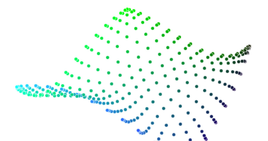
What about extra difficult varieties of topology? This can be a topic dearer to mathematicians than to sensible information analysts, however attention-grabbing low-dimensional buildings are often discovered within the wild.
Think about a set of factors that hint a hyperlink or a knot in three dimensions. As soon as once more, taking a look at a number of perplexity values provides probably the most full image. Low perplexity values give two utterly separate loops; excessive ones present a sort of international connectivity.
The trefoil knot is an attention-grabbing instance of how a number of runs have an effect on the end result of t-SNE. Under are 5 runs of the perplexity-2 view.
The algorithm settles twice on a circle, which a minimum of preserves the intrinsic topology. However in three of the runs it finally ends up with three completely different options which introduce synthetic breaks. Utilizing the dot coloration as a information, you’ll be able to see that the primary and third runs are removed from one another.
5 runs at perplexity 50, nonetheless, give outcomes that (as much as symmetry) are visually similar. Evidently some issues are simpler than others to optimize.
Conclusion
There’s a purpose that t-SNE has grow to be so common: it’s extremely versatile, and may typically discover construction the place different dimensionality-reduction algorithms can not. Sadly, that very flexibility makes it difficult to interpret. Out of sight from the person, the algorithm makes all kinds of changes that tidy up its visualizations.
Don’t let the hidden “magic” scare you away from the entire method, although. The excellent news is that by learning how t-SNE behaves in easy instances, it’s doable to develop an instinct for what’s happening.
[ad_2]
Source link
