

[ad_1]
How one can regulate CATE to think about prices related along with your therapies
Getting prospects to come back again to your small business is difficult. Within the age of aggressive trade incentives, manufacturers are spending a great deal of cash to get prospects to come back again within the door. A technique of convincing prospects to come back again to your organization is by interacting with them, exposing them to totally different commercials within the hopes of a brand new conversion.
Typically these commercials work, different occasions a buyer wants extra of an incentive. That is the place we will introduce reductions to the client to ensure that them to understand further worth in interacting with the model and abandon our equal prices commercial strategy. The plain problem with these reductions is that the model will lose worth on the transaction. That is the problem we’ll deal with: how do we all know which (if any) low cost to ship to the client to extend their conversion likelihood?
Some readers might have seen this downside is near the standard Uplift modelling state of affairs. We take some noticed therapies, evaluate them towards a management, and decide the remedy with the utmost Conditional Common Therapy Impact (CATE). Once we don’t have each the remedy and management noticed we estimate the counterfactual (what didn’t occur). To suit the Uplift framework we will rework the earlier query to: how will we regulate the CATE to think about the prices related to every remedy?
It is a downside that falls on us as Knowledge Scientists. We may also help the seasoned advertiser type by way of a group of commercials and reductions and work out what every buyer ought to see given beforehand noticed interactions. Main on this noticed knowledge, we may also help a enterprise or model resolve what the optimum technique is for interacting with prospects within the state of affairs outlined.
We begin with a whirlwind introduction to Uplift Modeling and Meta Learners, studying what every of these are and the way they clear up the equal prices downside. We then introduce the web worth CATE and present the minor modification we have to make to our Meta Learners to account for our prices. Along with the Meta Learner adjustment, we additionally take a look at an answer from CausalML referred to as the Counterfactual Worth Estimator (CVE) and the way this strategy solves the web worth downside. Lastly we take a look at some experiments and focus on some practicalities of how this could work in a manufacturing setting.
To ensure we’re all aligned on uplift modelling I’ve devoted this house to a short overview. Uplift Modelling is a framework underneath Causal Inference that focuses on figuring out the perfect remedy for particular person topics. The benefit to Uplift Modelling over conventional statistical studying methods is that we estimate the counterfactual results, the outcomes for a state of affairs that didn’t occur. Utilizing this estimation we will predict the remedy results for therapies the topic didn’t obtain, permitting us to reply the “What would have occurred if we did X?” query.
This measure of the distinction between the remedy and the management group is known as the Conditional Common Therapy Impact (CATE). To formalize this concept I’ll flip to some equations. We denote the end result for the topic as Y, the remedy as t, and the remedy identifier as j, with the particular case of j=0 because the management group. In our case Y is a binary variable that signifies if the person transformed or not. We situation the distinction on a column vector x which accommodates topic info, most vital of which might be buying behaviors. Utilizing this notation we’ve got the method offered under.
Now that we’ve got a desired worth to be taught, we’d like a technique that may estimate this worth. The most well-liked strategy to resolve this downside within the context of Uplift Modelling is thru the usage of Meta Learners. Meta Learners make use of the statistical fashions we’re all acquainted (i.e. Logistic Regression, LinearRegerssion, XGBoost, and so forth.) however reformat the issue to be taught an strategy to resolve for the CATE.
At their core, Meta Learners try to be taught the psuedo-effects for every remedy and wrap their studying round that estimate. The psuedo-effects are realized by taking the distinction between estimates of every remedy from statistical studying fashions and making comparisons towards noticed values and estimated values. On the finish of the Meta Learner workflow we output the CATE for every remedy.
For this text, it is just vital to know what CATE, not as a lot the way you be taught to estimate CATE. This rationalization of conventional uplift modelling to estimate the CATE is admittedly fast and never complete sufficient for a sensible utility of the strategy. I’d counsel this article for a great introduction and for a complete introduction for all issues associated to causal inference I counsel Causal Inference for the Brave and True.
As proven above, our price of CATE was solely capturing the conversion possibilities. Right here we shift views to think about a CATE that might be used to think about the whole worth of the conversion in addition to the price of the remedy used to activate the conversion.
In an effort to contemplate the worth, we have to introduce some new notation from Zhao and Harinen [1]. We introduce v because the anticipated worth of the transaction, s because the conversion price (i.e. the price of the remedy/low cost when activated), and c because the impression price (i.e. the price to indicate the remedy/low cost to the patron). Once more t represents a remedy and j represents the precise remedy, with j=0 being the particular case of the management group. Beneath we will see how we use these values to replace the CATE method to account for whole internet worth.
This method offers us some new flexibility in contemplating how you can apply therapies which have related prices. We are able to see that after we make comparisons of the Internet Worth CATE, we’ve got remedy results that think about pricing.
Primarily based on our above notion of internet worth CATE, it’s fairly trivial to increase the X-Learner to deal with this new basis of CATE. When utilizing the X-Learner one of many major steps is to be taught the pseudo-effects for the therapies given a prediction and the bottom fact. To do that we match a response mannequin (denoted by mu) for every remedy and calculate the distinction between the remedy group and the management group. For the values we don’t have (the counterfactuals) we estimate with a educated response mannequin utilizing a set of options for every particular person within the knowledge set. The usual pseudo results appear to be:
As mentioned above we need to seize internet worth in our pseudo-effects. We are able to accomplish this the best way that Zhao and Harinen [1] proposed with the identical modification we made to CATE above. For those who discover, the pseudo-effects are an estimate of CATE, how a lot better the remedy is than one other given a set of options in regards to the topic. By making the identical modification to the expectation we did above we will rework the net-value pseudo-effects as:
A pleasant results of modelling internet worth by way of the CATE is that that is the one adjustment to the X-Learner we have to make. Since CATE is already a steady variable the next fashions that have to be educated to preidct CATE are outfitted to deal with the regression job.
There are another approaches to think about internet worth within the comparability. One which we’ll contemplate right here is the answer carried out in CausalML, a python library maintained by Uber. Their answer, the Counterfactual Worth Estimator (CVE), innovates on the identical thought of calculating internet worth CATE, however takes a barely totally different strategy to the place the calculation occurs.
CVE is a put up modelling optimizer that takes inputs from a couple of fashions to estimate the web worth CATE. The primary mannequin used is a conversion likelihood mannequin. This mannequin is used to foretell the likelihood the topic will convert given their options and the remedy they obtain.
The following mannequin educated for the CVE is any learner that may predict CATE. The CATE is mixed with the conversion possibilities to find out what the convergence likelihood is underneath the remedy state of affairs towards the counterfactual. This calculation appears to be like like this:
The following mannequin educated for the CVE is the anticipated conversion worth predictor. Relying on the state of affairs this mannequin won’t be crucial. For those who can simply sub historic spending for a way a lot the person will spend then that may be a viable possibility. Nevertheless, you probably have some info on how the person interacts along with your model or how a lot they’re more likely to spend on their subsequent transaction then you possibly can mannequin that by way of a regression downside.
At this level we’ve got the entire predicted values we have to use the web worth CATE described above to optimize which remedy is probably going to present the biggest internet worth payout. For extra info on this strategy you possibly can take a look at the data offered in [2]. Latter within the article we’ll discover the idea additional with code.
Right here we’ll step by way of an instance of how one can apply the strategies mentioned to date. We’ll make use of some helper capabilities from CausalML and in addition adapt one among their notebooks for the instance. We’ll additionally consider precisely as they did of their pocket book. To see their demo, take a look at this link.
The metric we’ll use is a possible earnings heuristic for what our common earnings would have been if we had employed this remedy project coverage on the earlier batch of knowledge. On the maintain out knowledge we match all instances the place our remedy is the same as the noticed remedy. When these are equal we discover the common worth of these people. To additional make clear I wrote some hypothetical SQL under that will present how that is calculated, with the column names following the variables we’ve mentioned all through the article.
SELECT AVG((expected_value - conversion_cost) * conversion - impression_cost)
FROM preds_and_ground_truth
WHERE predicted_treatment = ground_truth_treatment;
Very first thing we have to do is create our knowledge. For this instance we’ll use two therapies and a management group. I set the positive_class_proportion=0.1 which represents a conversion charge of 10%. This quantity could also be totally different primarily based in your state of affairs so if you happen to’re simulating be certain to select this accordingly.
df, X_names = make_uplift_classification(
n_samples=5000,
treatment_name=["control", "treatment1", "treatment2"],
positive_class_proportion=0.1,
)
The following factor we’ll do right here is create our price associated capabilities. The primary would be the anticipated worth, which I created as a perform of one of many irrelevant options. This function has no affect on the conversion, so it exams our strategies capacity to calculate anticipated spend when making the optimization.
df['expected_value'] = np.abs(df['x6_irrelevant']) * 20 + np.random.regular(0, 5)
Now we’ll create the entire price info utilizing the helper capabilities from CausalML. We’ll create our conversion price array cc_array , our impression price array ic_array , and get the circumstances (our therapies). The conversion worth array is simply the anticipated worth we created above.
# Put prices into dicts
conversion_cost_dict = {"management": 0, "treatment1": 2.5, "treatment2": 10}
impression_cost_dict = {"management": 0, "treatment1": 0, "treatment2": 0.02}# Use a helper perform to place remedy prices to array
cc_array, ic_array, circumstances = get_treatment_costs(
remedy=df["treatment_group_key"],
control_name="management",
cc_dict=conversion_cost_dict,
ic_dict=impression_cost_dict,
)
# Put the conversion worth into an array
conversion_value_array = df['expected_value'].to_numpy()
Subsequent we will create the precise worth array. That is the worth of the transaction following the identical method for our expectation above.
actual_value = get_actual_value(
remedy=df["treatment_group_key"],
observed_outcome=df["conversion"],
conversion_value=conversion_value_array,
circumstances=circumstances,
conversion_cost=cc_array,
impression_cost=ic_array,
)
Random Coverage
The primary coverage we’ll take a look at is randomly assigning therapies to totally different topics. This might look one thing like this:
test_actual_value = actual_value.loc[test_idx]
random_treatments = pd.Sequence(
np.random.selection(circumstances, test_idx.form[0]), index=test_idx
)
test_treatments = df.loc[test_idx, "treatment_group_key"]
random_allocation_value = test_actual_value[test_treatments == random_treatments]
Finest Therapy Coverage
The following coverage is taking the remedy that has the very best Common Therapy Impact (ATE). This doesn’t contemplate context of the topic in any respect.
best_ate = df_train.groupby("treatment_group_key")["conversion"].imply().idxmax()actual_is_best_ate = df_test["treatment_group_key"] == best_ate
best_ate_value = actual_value.loc[test_idx][actual_is_best_ate]
Finest Doable
The absolute best coverage is an oracle we will look in direction of to evaluate how our fashions evaluate. This mannequin is one which considers solely instances through which we misplaced no worth. That is the case when the topic was within the management group or they transformed after we despatched them one among two therapies.
test_value = actual_value.loc[test_idx]
best_value = test_value[test_value >= 0]
X Learner
Right here we’ll use only a plain X Learner with no price optimization. The X Learner I exploit right here is one which I carried out, so if you want to experiment with that I included a hyperlink under to my repo under.
xm = XLearner()
encoder = {"management": 0, "treatment1": 1, "treatment2": 2}
X = df.loc[train_idx, X_names].to_numpy()
y = df.loc[train_idx, "conversion"].to_numpy()
T = np.array([encoder[x] for x in df.loc[train_idx, "treatment_group_key"]])xm.match(X, y, T)
To get the perfect remedy in line with the XLearner we will get the anticipated CATE values and take the remedy with the max worth by way of an argmax on the dataframe.
X_test = df.loc[test_idx, X_names].to_numpy()
xm_pred = xm.predict(X_test).drop(0, axis=1)
xm_best = xm_pred.idxmax(axis=1)
xm_best = [conditions[idx] for idx in xm_best]actual_is_xm_best = df_test["treatment_group_key"] == xm_best
xm_value = actual_value.loc[test_idx][actual_is_xm_best]
Counterfactual Worth Estimator
To make use of the CVE from CausalML we have to first prepare a couple of fashions. The primary mannequin is the conversion classifier. That is only a straight ahead classification downside. We use the classifier to foretell the likelihood of changing given their remedy publicity and different info we might learn about them.
proba_model = lgb.LGBMClassifier()W_dummies = pd.get_dummies(df["treatment_group_key"])
XW = np.c_[df[X_names], W_dummies]
proba_model.match(XW[train_idx], df_train["conversion"])
y_proba = proba_model.predict_proba(XW[test_idx])[:, 1]
The following mannequin we have to prepare is a mannequin to foretell the anticipated worth of the visitor’s conversion. That is one other straight ahead downside, this time regression.
expected_value_model = lgb.LGBMRegressor()
expected_value_model.match(XW[train_idx], df_train['expected_value'])
pred_conv_value = expected_value_model.predict(XW[test_idx])
The opposite worth we use for this mannequin is the anticipated CATE values. Within the earlier step we match an X-Learner, which predicted the CATE for us. Now we will optimize our actions utilizing the CVE.
cve = CounterfactualValueEstimator(
remedy=df_test["treatment_group_key"],
control_name="management",
treatment_names=circumstances[1:],  # idx 0 is management
y_proba=y_proba,
cate=xm_pred,
worth=pred_conv_value,
conversion_cost=cc_array[test_idx],
impression_cost=ic_array[test_idx],
)
CVE is a non-parametric optimizer. Because of this we don’t be taught any weights after we use the CVE. As an alternative, we take the values we’ve got already realized and optimize them for exterior prices when predicting the motion. Beneath is an instance of how we will get the perfect actions from CVE.
cve_best_idx = cve.predict_best()
cve_best = [conditions[idx] for idx in cve_best_idx]
actual_is_cve_best = df.loc[test_idx, "treatment_group_key"] == cve_best
cve_value = actual_value.loc[test_idx][actual_is_cve_best]
Internet Worth Optimized X-Learner
The following coverage we’ll take a look at is the X-Learner once more, however this time one which considers the Internet Worth CATE as an alternative of the vanilla CATE. This is similar X-Learner from earlier than, the one from my repo. If you need to experiment with it please take a look at the repo linked under.
nvex = XLearner(ic_lookup=ic_lookup, cc_lookup=cc_lookup)X = df.loc[train_idx, X_names].to_numpy()
y = df.loc[train_idx, "conversion"].to_numpy()
T = np.array([encoder[x] for x in df.loc[train_idx, "treatment_group_key"]])
worth = df.loc[train_idx, "expected_value"].to_numpy()
nvex.match(X, y, T, worth)
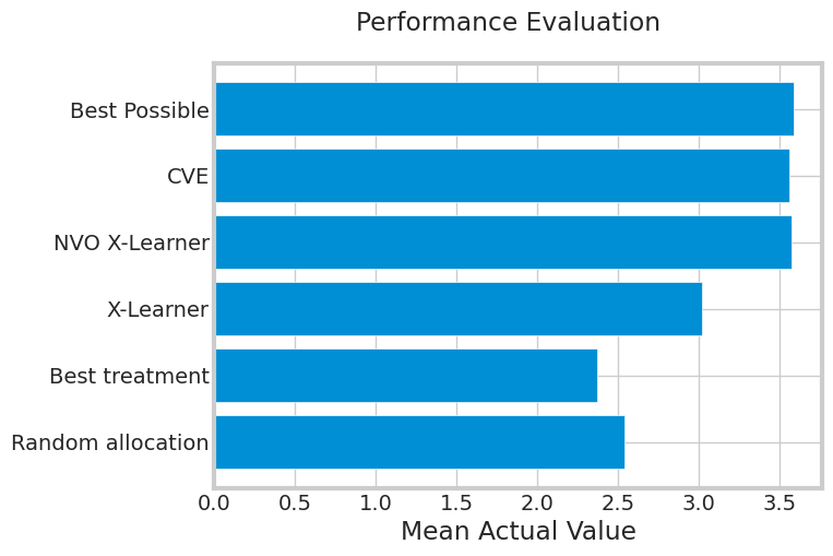
Beneath we will see the outcomes of every coverage for imply worth within the testing set. As we anticipated the strategies that optimized worth within the distribution of therapies outperformed people who didn’t contemplate worth. Random Allocation and Finest Therapy function good baseline measures however don’t present efficiency that make them a aggressive naive methodology. The X-learner is an efficient enchancment over the naive strategies however does to carry out in addition to the strategies that think about internet worth. The most effective efficiency comes from the Internet Worth Optimized (NVO) X-Learner and the CVE. It’s because these strategies are optimized for the web worth which is the metric we’re measuring them towards.

To measure success in a proper marketing campaign I’d suggest a barely extra concerned strategy following a backtesting paradigm. For these unfamiliar, backtesting includes testing an algorithm on historic knowledge utilizing a holdout set on a cutoff date. Suppose you’ve gotten 90 days of knowledge. A backtesting evaluation of a technique/algorithm would contain coaching on 45 and testing on the subsequent 45 days, then incrementing the coaching set by some fastened worth of days and repeating the coaching and validation downside. Right here we will take the identical strategy with our methodology and take a look at how the algorithm performs on historic increments.
When executing a marketing campaign like this, your fashions are solely nearly as good as your knowledge. Random knowledge is pricey and sure not possible for the entire of your knowledge, however it is very important have some random knowledge. When distributing your therapies, make sure to acquire some subsample that’s randomly assigned. This knowledge is greatest to make use of for validation functions to be sure that the algorithm you educated hasn’t realized any tendencies that come from imbalances in how the therapies are distributed.
For these involved about coaching on observational knowledge there are a couple of pure methods it’s accounted for. Within the X-Learner we be taught a propensity mannequin for remedy project. When contemplating the remedy impact we be taught a weighted common over the chance the person was assigned to that remedy group. For extra info I’d counsel taking a look at formulation (10), (11) and (12) from [1].
Observational knowledge imbalances can be accounted for within the conversion mannequin and the regression mannequin. By measuring accuracy inside remedy teams for the conversion and anticipated worth fashions, we will be certain the info isn’t biased to anybody group. If the outcomes do change into biased there are many sampling methods that might be used to repair this downside (this is an efficient instance of one thing simple.)
Right here we noticed an introduction on how you can optimize worth when distributing therapies. We mentioned how this downside is often dealt with, which included a whirlwind tour of Uplift Modelling and launched ATE and CATE. Then we modified how CATE was calculated to incorporate worth, conversion price, and impression price within the expectation to be taught the web worth CATE. We moved on to take a look at an current answer offered by CausalML referred to as the Counterfactual Worth Estimator and noticed how that accounted for internet worth CATE. Lastly we stepped by way of the pocket book from CausalML and prolonged with our Internet Worth Optimized X-Learner.
You’ll be able to entry my repo here!
You’ll be able to entry the unique pocket book from CausalML here!
All photographs belong to the Writer until in any other case famous.
[ad_2]
Source link
