Working with Confidence Intervals – KDnuggets

Picture by Editor

In knowledge science and statistics, confidence intervals are very helpful for quantifying uncertainty in a dataset. The 65% confidence interval represents knowledge values that fall inside one normal deviation of the imply. The 95% confidence interval represents knowledge values which might be distributed inside two normal deviations from the imply worth. The boldness interval may also be estimated because the interquartile vary, which represents knowledge values between the twenty fifth percentile and the seventy fifth percentile, with the fiftieth percentile representing the imply or median worth. 

On this article, we illustrate how the arrogance interval will be calculated utilizing the heights dataset. The heights dataset accommodates female and male peak knowledge.

First, we generate the chance distribution of the female and male heights.

# import mandatory libraries
import numpy as np
import pandas as pd
import matplotlib.pyplot as plt
import seaborn as sns

# get hold of dataset
df = pd.read_csv('https://uncooked.githubusercontent.com/bot13956/Bayes_theorem/grasp/heights.csv')

# plot chance distribution of heights
sns.kdeplot(df[df.sex=='Female']['height'], label="Feminine")
sns.kdeplot(df[df.sex=='Male']['height'], label="Male")
plt.xlabel('peak (inch)')
plt.title('chance distribution of Male and Feminine heights')
plt.legend()
plt.present()

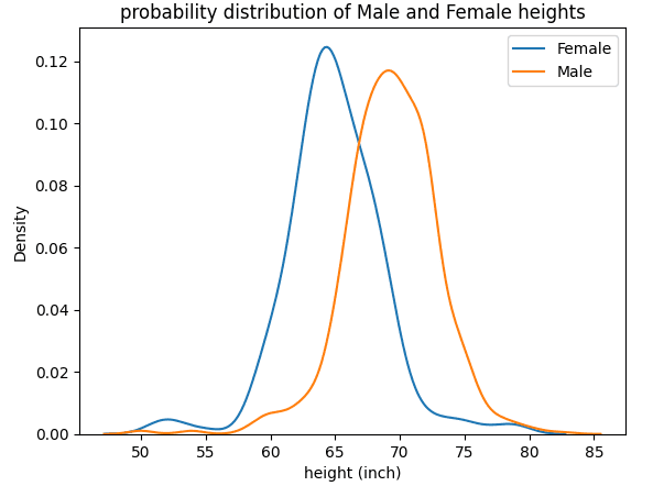
Likelihood distribution of female and male heights | Picture by Writer.

From the determine above, we observe that males are on common taller than females.

The code under illustrates how the 95% confidence intervals for the female and male heights will be calculated.

# calculate confidence intervals for male heights
mu_male = np.imply(df[df.sex=='Male']['height'])
mu_male

>>> 69.31475494143555

std_male = np.std(df[df.sex=='Male']['height'])
std_male

>>> 3.608799452913512

conf_int_male = [mu_male - 2*std_male, mu_male + 2*std_male]
conf_int_male

>>> [65.70595548852204, 72.92355439434907]

# calculate confidence intervals for feminine heights
mu_female = np.imply(df[df.sex=='Female']['height'])
mu_female

>>> 64.93942425064515

std_female = np.std(df[df.sex=='Female']['height'])
std_female

>>> 3.752747269853828

conf_int_female = [mu_female - 2*std_female, mu_female + 2*std_female]
conf_int_female

>>> [57.43392971093749, 72.4449187903528]

One other technique to estimate the arrogance interval is to make use of the interquartile vary. A boxplot can be utilized to visualise the interquartile vary as illustrated under.
 

# generate boxplot
knowledge = checklist([df[df.sex=='Male']['height'],   
             df[df.sex=='Female']['height']])

fig, ax = plt.subplots()
ax.boxplot(knowledge)
ax.set_ylabel('peak (inch)')
xticklabels=['Male', 'Female']
ax.set_xticklabels(xticklabels)
ax.yaxis.grid(True)
plt.present()

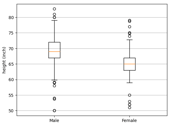
Field plot exhibiting the interquartile vary.| Picture by Writer.

The field exhibits the interquartile vary, and the whiskers point out the minimal and most values of the info, excluding outliers. The spherical circles point out the outliers. The orange line is the median worth. From the determine, the interquartile vary for male heights is [ 67 inches, 72 inches]. The interquartile vary for feminine heights is [63 inches, 67 in]. The median peak for males heights is 68 inches, whereas the median peak for feminine heights is 65 inches.

In abstract, confidence intervals are very helpful for quantifying uncertainty in a dataset. The 95% confidence interval represents knowledge values which might be distributed inside two normal deviations from the imply worth. The boldness interval may also be estimated because the interquartile vary, which represents knowledge values between the twenty fifth percentile and the seventy fifth percentile, with the fiftieth percentile representing the imply or median worth.
 
 
Benjamin O. Tayo is a Physicist, Knowledge Science Educator, and Author, in addition to the Proprietor of DataScienceHub. Beforehand, Benjamin was educating Engineering and Physics at U. of Central Oklahoma, Grand Canyon U., and Pittsburgh State U.